Week 9 - Parametric study on Gate valve.
Aim: - Parametric analysis of gate valve to simulate valve lift also to calculate flow factor and flow coefficient.
Objective: -
- To study the functioning of gate valve in flow industries.
- To pre-process the geometry for simulation.
- To defined input parameter for the simulation in space-claim.
- To mesh the geometry with better mesh quality for converged results.
- To simulate the valve lift from 10% to 80% opening.
- To calculate the mass flow rate at the outlet of pipe.
- To calculate flow coefficient and flow factor.
- To plot flow coefficient and flow factor with respect to valve lift.
Introduction: -
In most of the industries where water or other liquid are used for the treatment processing there should be controlling of flow medium as and when required. Pipes are used to transport the medium in and out of the system for processing and other removal of waste. To monitor and regulate the flow in the pipes there are pipe valve in most of the cases gate valve which also known as sluice valve. It is a valve that opens by the barrier called gate out of the path of flow of fluid. This valves are installed along the pipe axis and takes very little place to mount on the pipe, when open this valve does not restrict any of the flow of fluid inside the pipe. The gate which is a barrier has his faces parallel but most commonly are in the wedge shape to put pressure on the sealing surface. The valve assembly has numerous part within it which is shown by below image:
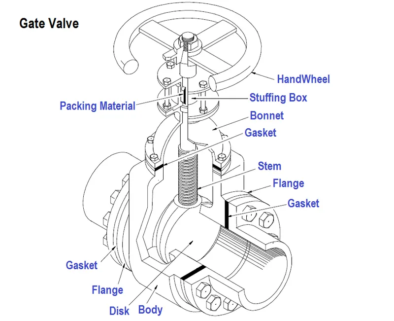
The valve body is inserted in between the pipe and its flange is bolted to the pipe flange where it has to be installed. Between the two flanges the gasket is applied to restrict any leakage between the pipes. The gate body or disk is connected to screw which is further connected to the wheel to lift up and down the gate body to the surface of valve body. To ensure the air tight arrangement the bonnet is bolted to the main body of valve with gasket inside it. The stem of gate valves is categorizing in two different section one is rising stem and other one is non-rising stem. The non-rising stem valve are fixed and rotate inside the valve body. This type of flow valve restricts some amount of fluid flow. The non-rising gate valve are used where the vertical space for the installation is limited also they are used where the water is pressure minimum. The high water pressure gate valve is having some by-pass mechanism to counter the pressure applied by fluid on the gate disk so that vibration is at minimum level.
The use of the gate valve is to shut off the flow completely. When the gate is fully open it often restrict any fluid flow in the pipes. The material used for gate valve is cast iron, cast carbon steel, stainless steel and alloy steels. The most of the control valve are produced before installation and with high factor safety. This valve is designed on the basis of future load perspective in the plant for monitoring the fluid flow. A correctly sized control valve can provide significant quantifiable savings and increase process availability which eventually reduce the maintenance costs.
The sizing of this valves are very important and has to be accepted on the mathematical method which are describe in ISA-75.01.01-2007 – Flow Equations for Sizing Control Valves. The most common parameters in the valve sizing are flow coefficient and flow factors.
Flow Coefficient (Cv)
Flow coefficient is the term associated with the lift of gate or disc in controlling valve which is part of sizing while designing the valves. The flow coefficient denoted as Cv is a measure of the capacity of the valve body and trim. A valve Cv can be described as the number of gallons per minute (GPM) at 15.5℃ that will pass through a valve with an associated pressure drop of 1 psi. In easy term of definition, a fully open valve with a Cv of 14GPM/psi passes 14GPM of fluid with 1psi of pressure drop. The flow coefficient is used to determine the valve size that will best allow the valve to pass the required flow rate while providing stable control of the process fluid. Most of the manufacturer provide the Cv data for the valves in catalogues.`Kv=Q√(SG)/(ΔP)`
The Cv of the valve has to be calculated correctly or the valve performance will get lower along the service life of valve. If the Cv of the valve too small, the trim inside the valve will be undersized resulting in system to be starved of the process fluid. Undersized valve has higher pressure drop across the valve to maintain the adequate flow and shows low fluid capacity. The undersized control valve generally cannot deliver sufficient flow rates under maximum loads conditions. If the Cv calculate for the system is too high, it results in larger oversized control valve is usually selected. The issue with oversized valve such as larger cost, weight and size and in throttling service the significant instability is occurred. Oversized valve is quite common and are highly sensitive to operating conditions with the even the smallest adjustment in valve position causing significant changes in the fluid flow rate.
The equation which is used to calculate the flow coefficient is given as:
`Cv=Q√(SG)/(ΔP)`
where,
Q is mass flow rate in US gallons per minute.
SG is specific gravity of liquid (water = 1)
∆P is pressure drop across the valve expressed in psi
Flow Factor (Kv)
Flow factor is metric equivalent of the flow coefficient Cv is based on the SI system. The difference between the flow coefficient and flow factor is that flow factor is used outside the united states. It is same as flow coefficient just the unit of measurement is different.
`Kv=Q√(SG)/(ΔP)`
where,
Q is mass flow rate expressed in m3/hr.
SG is specific gravity of liquid (water = 1)
∆P is pressure drop across the valve expressed in bar.
There is a co-relation between the flow coefficient and flow factor which is given as:
`Cv=1.16Kv`
`Kv=0.862 Cv`
Solution Approach and Methodology: -
The main aspect in the solution approach for this problem is the use of parametrization in the project schematic of ANSYS. The pre-processing of the simulation is most important part for the simulation and has to be precise to have any error free simulation for rest of the case. The solution approach for the problem is to have pressure based solver with steady state approach to solve the simple flow problem. The flow in pipes are mostly governed by pressure difference hence rather than using velocity as inlet for flow there will be pressure inlet and pressure outlet boundary conditions. The flow in the pipes are mostly turbulent in nature hence K-epsilon realizable with scalable wall functions is used as viscous formulation. The working fluid will be water for this simulation.
The methodology which will be used in this simulation is to create the input parameter in space-claim and output parameter in FLUENT. The input parameter will be the valve lift height in assembly and it has to be update as new input parameter will enter for simulation. The output parameter is the mass flow rate at outlet which is defined in post-processing. The two main output required to calculate the flow coefficient and flow factor are mass flow rate and pressure drop between the inlet and outlet. The main advantage of parametric simulation is that; it will lower the pre-processing time for each case of the simulation. If the simulation cases are greater in number and number of variable to change for simulation are lower, then use of parametric simulation is one of the best option for engineers. The most industrial simulations are based on the parametric study which are used in numerous problem where product design and product optimization with respect to working conditions are main focus.
For this simulation the fluid body is need to be create in the solid assembly by initially rising the gate valve body by 10mm in height. This height of valve body has to be parametrize with respect to further extent of height in simulation. Space-claim is well suited for automatically update of geometry for simulation as compare to design modeler. The design modeler has edge when define of parameter but making an update with internal geometry is very difficult. The meshing of the problem is another aspect for this simulation. The internal flow simulation with restriction in the path of flow should have better mesh characteristic near the valve body. If the elements get too coarse in this area will result to diverged solution for problem. Use of correct method and sizing parameter become important for such simulations. The best aspect of parametrization is that, it will allow any input parameter to define for problem from geometry modelling, meshing and upto solver setup. Changing number of variable for simulation of any product while designing provide more accurate results for the final development.
Pre-processing – Geometry: -
The main aspect of simulation is to create the fluid volume inside the Gate valve assembly with respect to changing height of valve disc inside body. The image of Gate valve is shown below:
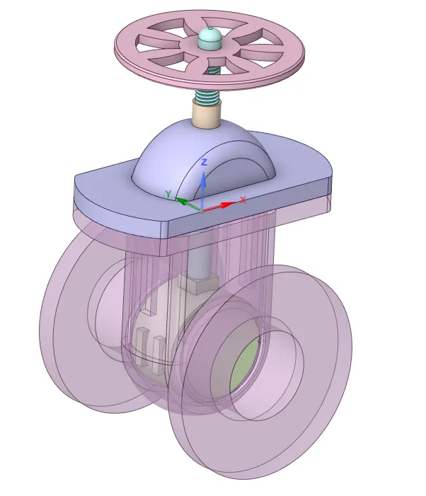
In above image, the valve disc is present inside the valve body. There is bonnet at the top from which a valve stem protrudes outward and connected to wheel. The stem is connected to the valve disc. For the initial simulation this valve body has to be raise by 10mm to create the fluid volume inside. This can be done by hiding lower body of Gate valve and using move tool in space-claim. The following image showing the lifting of gate valve.
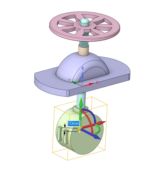
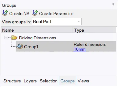
With the new version of space-claim there is no option to directly making the dimension as parameter as it was in previous versions. To make the dimension as parameter user need to navigate to group section which is below the tabs of space-claim. In the group section there is option to create parameter which need to be click and after that first group of parameter with dimension of 10mm will be added automatically as it was showing the working area of space-claim. The image of group section is shown below:
After completion of group section, the lower valve body has to checked in to reshow in the assembly for making of a fluid volume inside Gate valve. The length of inlet and outlet of Gate has to increase in order to lower the effect of reverse flow inside the domain. The reverse flow from outlet is start when the fluid domain is not big enough to calculate the flow condition accurately. The extension of inlet face and outlet face of Gate valve is done by pull command in space-claim. In pull command one has to select the face which need to be pulled or extent in forward direction or opposite direction. After completion of operation for pull tool the final geometry is shown below:
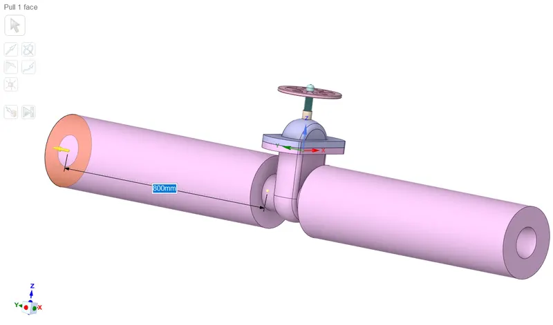
It can be seen that in above image the length of inlet and outlet is increase by 800mm in both directions. After that it is easy to become extract fluid volume in the Gate valve. Before doing that it is recommended to hide the bonnet part from the assembly to select the boundary edges of the parts which is shown in below image.
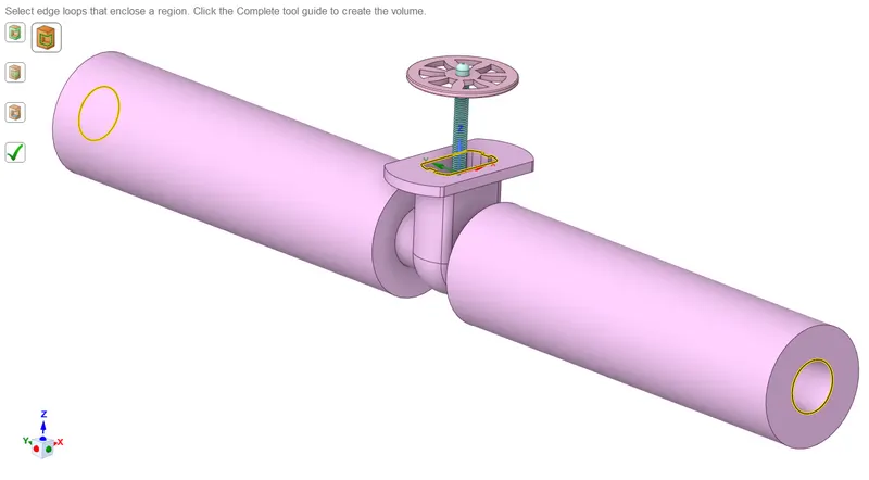
In above image three edges are selected to complete the volume extract operation by selecting edge loop command to enclose a region. This command best possible volume extract method for whole geometry. If geometry having any missing faces and edges, then it became very difficult for user to create the internal volume. This can be avoided by checking the geometry first for missing edge or face. After completing the operation, the internal volume of the Gate valve assembly is shown below:
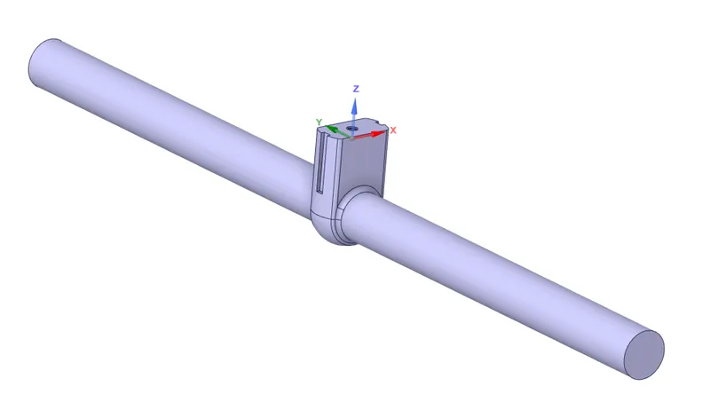
After removing the fluid volume from Gate valve, next thing is to make adjustment of height for each of simulation and update of geometry with respect to parameter. This can be done by again raising the gate disc body by 10mm in height but hiding the bonnet and wheel from assembly. In this case use of section plane plays big part for understanding of operation. The cross section view of geometry with internal volume and assembly parts is shown below:
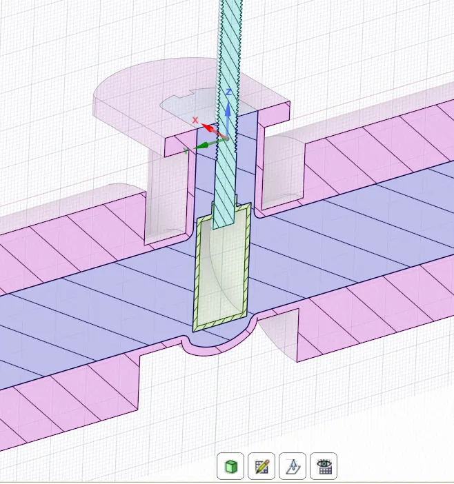
In above section view only valve disc, valve body and spindle or stem is visible with internal fluid volume. The main aspect of this operation is to modify the internal volume automatically for each valve lift height. The move tool in space-claim has to be used again for lifting the valve disc by 10mm again. This is shown below:
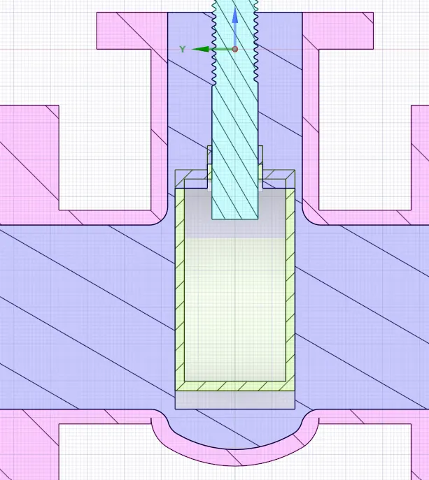
From above image it is clearly seen that, the gate disc has been raised by 10mm distance in height but the fluid volume is not updated also there is some interference created between the solid gate disc and internal fluid volume. This has to be corrected and update for each of 10mm increase of height of gate disc for particular simulation case. It can be done from the structure tree of space-claim. The user has to right click on the volume which has created in the first place by using volume extract operation. After right clicking the volume component there is option of update the volume body in context which allows user to update the volume body using current body arrangements. After selecting this option, the final geometry is shown below:
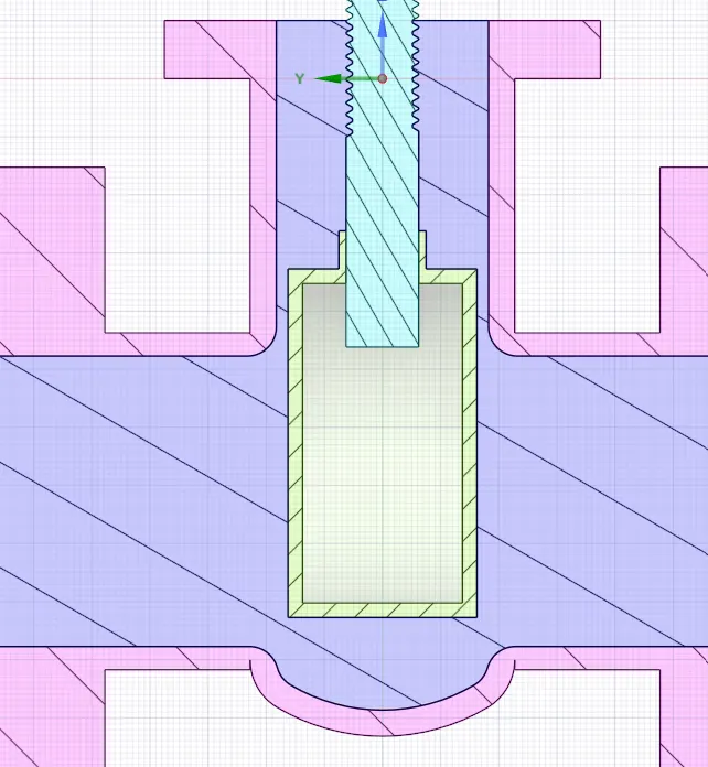
The first case parameter dimension of the simulation is 10mm hence it is important to again lower the height of the valve disc and perform similar operation for proceeding towards meshing.
Pre-processing – Meshing -
After completing the geometric pre-processing with Gate valve assembly, the meshing has to be done. Before transferring the geometry from space-claim to meshing, all the parts of assembly except internal fluid volume has to be suppressed for physics as they are not required in the simulation. In meshing the both tetrahedral mesh and hexahedral mesh setup has been used but it seems that tetrahedral mesh have good effect on the first two simulations with gate disc valve height upto 20mm increment. For onward 20mm increment the mesh size has to be lowered and was creating difficulty for the convergence.
The second mesh setup is carried out by putting hexahedral mesh into the account. The creation of hexahedral mesh is done by the meshing method called body fitted Cartesian with the global size of 4mm. As the simulation is done in academic version the cells are limited for problem. The mesh for problem is shown below:
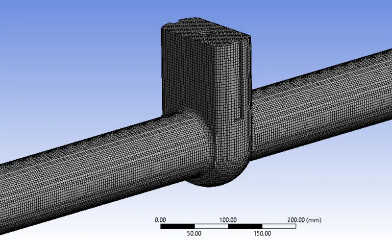
The section view of mesh is shown below:
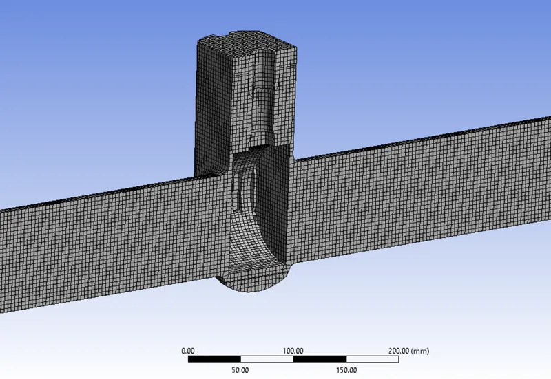
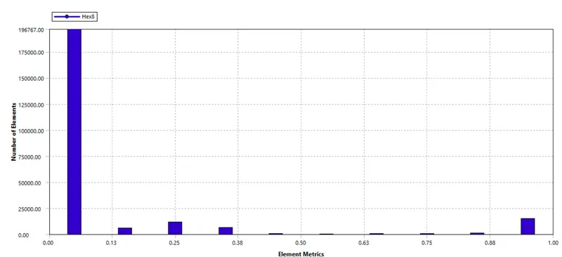
The total number element created in the process are 237738 and number of nodes are 266096. The mesh which has been created should also have better meshing quality. The mesh quality skewness is maximum 0.9 is achieved for around 10000 elements which is less than that of 20% of total elements hence can be accepted. The graph of skewness quality is shown below:
Pre-processing – FLUENT Setup.
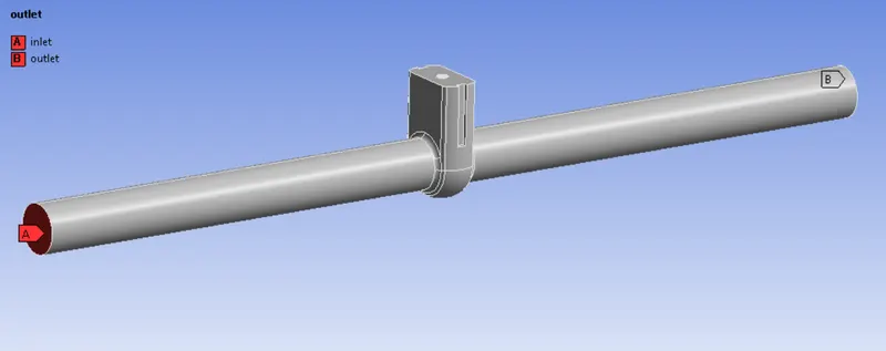
Before starting setup of the FLUENT it is important to create named selection in workbench which will act as boundary conditions for problem. The problem has only two named selections i.e. inlet and outlet which are shown below:
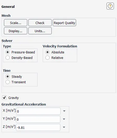
The flow phenomenon of the simulation is under the gravity and as the velocity of fluid flow is medium and there are no compressibility effects are considered in simulation then pressure based solver is used for problem. The flow is not time dependent hence steady state approach is used. The general setup for the simulation is shown below:
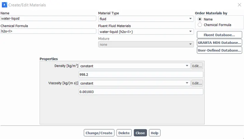
For this case the flow inside pipe is considered as turbulent hence the Reynolds number is more than 2000 for this case. For the pipe flow Reynolds number greater than 2000 means the turbulent flow. The viscous model which is used for this case is K-epsilon model with realizable method and using scalable wall function to capture near wall treatment of turbulent flow phenomenon. The working fluid for this case is considered as water which can be added in to the material data from fluent database. The properties of water are shown below:
In cell zone condition where only one volume is present need to be edited and set as the working fluid as water. The flow inside the pipes are mostly occurred due to pressure drop, hence this problem is treated as pressure inlet and outlet conditions rather than velocity inlet and pressure outlet boundary conditions. To change the inlet boundary condition from velocity inlet to pressure inlet one has to choose pressure inlet from the drop down menu of boundary condition selection. The pressure inlet of 10 Pascal is used and is shown below:
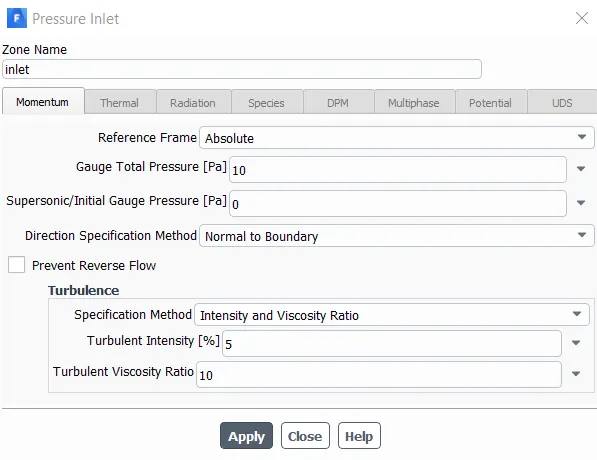
The outlet boundary condition is considering as pressure outlet with atmospheric pressure at end. The solution methods are treated as by default by FLUENT and there were no changes are made except turbulent dissipation rate and turbulent kinetic energy is treated as second order upwind function. The image for outlet boundary condition is shown below:
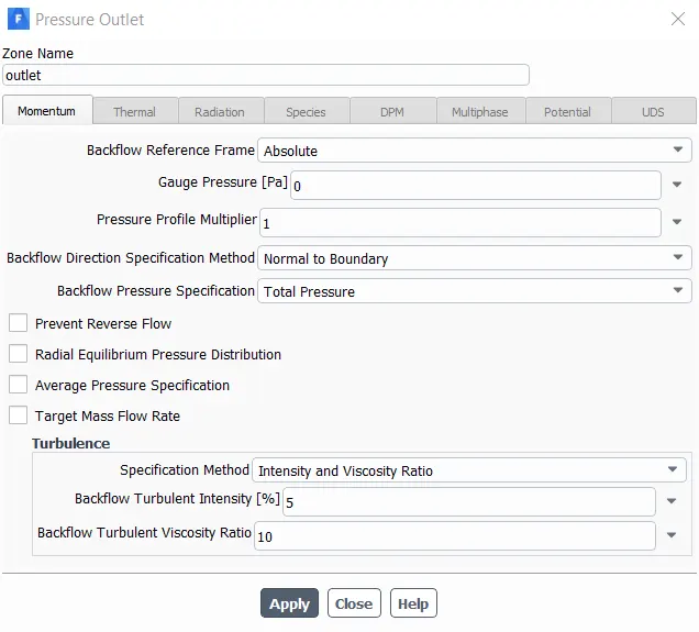
From the standard initialization method, the initial value for simulation is plotted from inlet boundary conditions. The method will provide the data for inlet velocity for which fluid flow is going to travel which is 0.1415 m/s. From this value we can validate that the flow inside pipe is turbulent by using Reynolds number equation which is given as:
`Re=(ρ*V*D)/μ=(998.2*0.1415*0.1)/0.001003=14087.14`
The output parameter which is required for calculation of flow coefficient and flow factor is mass flow rate. This parameter is need to evaluated with respect to every increment of rising gate disc in valve assembly. Hence after solution initialization the output report is generated of mass flow rate which is calculated at the outlet. The inlet mass flow rate is calculated using given empirical relation:
`Flow Rate=ρ A V=998.3*100*0.1415=1.0191 (kg)/s`
In above equation we calculating mass flow rate rather than volumetric mass flow rate which is different entity. The check for simulation is to have same or lower mass flow rate which has been calculated at the inlet. If the mass flow rate is greater than inlet, then the simulation has some errors which need to be look out. The report definition for mass flow rate at outlet is shown below:
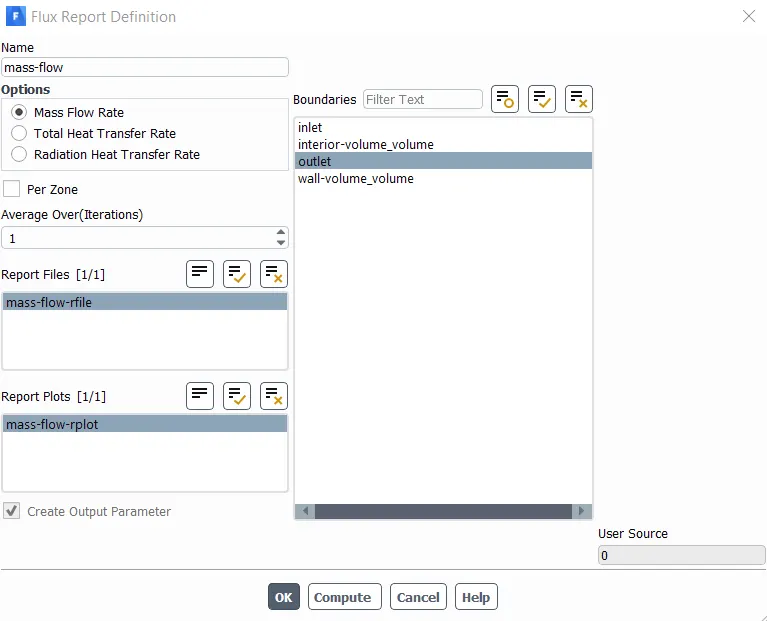
It is important to check the create output parameter box in the window or else it will not be recorded for each simulation with respect to input parameter. The parameter window before simulation will be seen as:
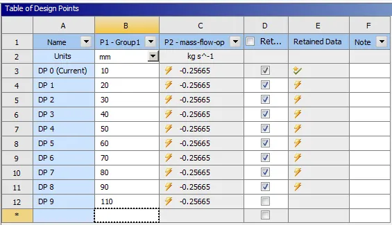
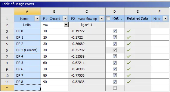
From this above parameter window it can be seen that the simulation will be running from 10mm height to 80mm which is desired with the problem, but additional increment is added for checking of final mass flow rate when valve is fully opened. It is important to check the retain data mark in parameter or else if we update the all points and want to get result from specific case the FLUENT will not have the result for that particular case to show.
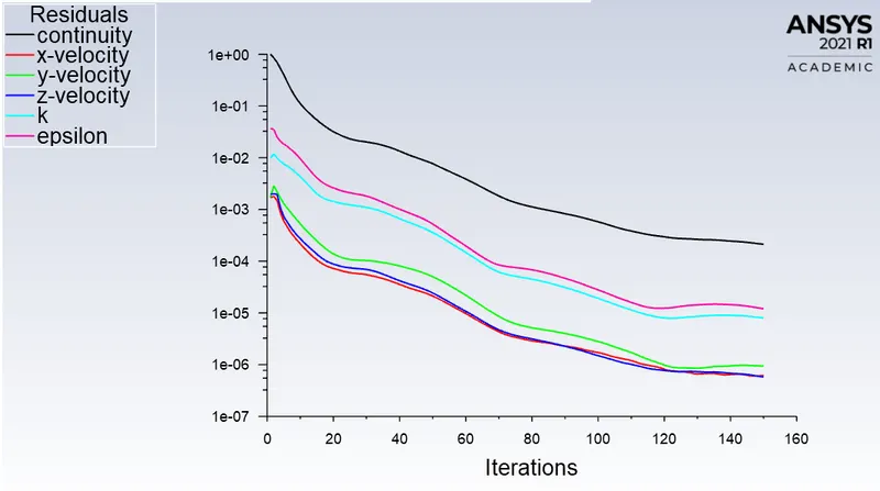
The number of iteration required for simulation are only 78 as it was converged early for simulation, to get good prospect of result the iterations are done for 150 without convergence factor. To check the animation of flow inside the gate valve an animation is created on a plane which is parallel to axis of flow.
Result – Lift 10mm
1) Residuals
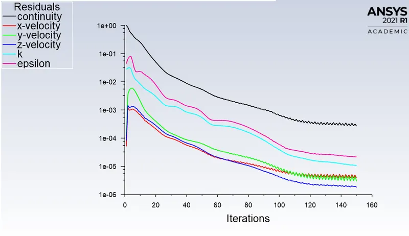
2) Mass flow rate
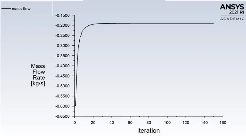
3) Pressure Result
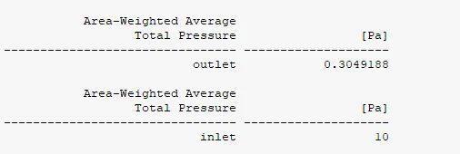
4) Flow coefficient
Mass flow rate = 0.1922 kg/s
Mass flow rate in US gallons per minute = 3.05 GPM
Inlet pressure in psi = 0.00145 psi
Outlet pressure in psi = 4.42e-5 psi
Pressure drop = Inlet pressure – Outlet pressure = 0.001405 psi
Specific gravity of water = 1 gm/cc.
`Cv=3.05√(1/0.001405)=81.346`
5) Flow Factor
Mass flow rate = 0.1922 kg/s
Mass flow rate in m3/hr = 0.69 m3/hr
Inlet pressure in bar = 1e-4 bar
Outlet pressure in bar = 3e-6 bar
Pressure drop = Inlet pressure – Outlet pressure = 0.000097 bar
Specific gravity of water = 1 gm/cc.
`Kv=0.69√(1/0.000097)=70.05`
6) Velocity Contour
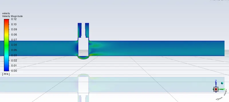
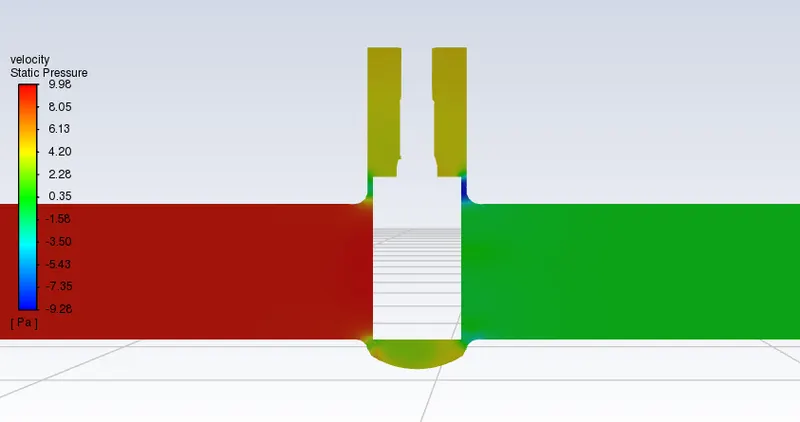
7) Pressure contour
8) Velocity Animation
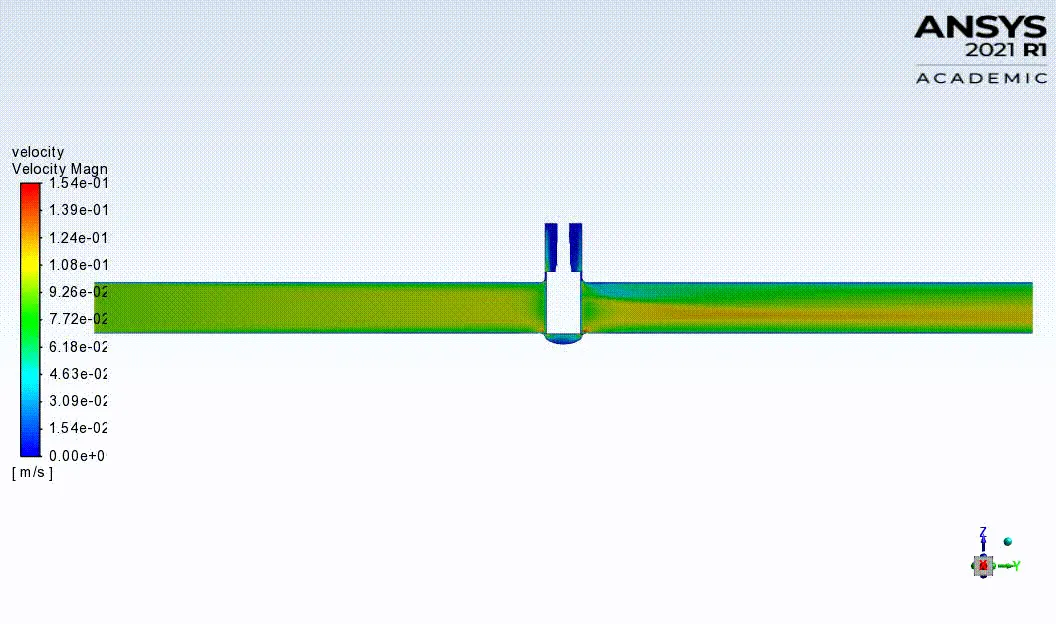
Result – Lift 20mm
1) Residuals
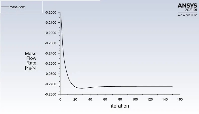
2) Mass flow rate
3) Pressure result
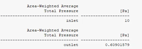
4) Flow Coefficient
Mass flow rate = 0.2722 kg/s
Mass flow rate in US gallons per minute = 4.31 GPM
Inlet pressure in psi = 0.00145 psi
Outlet pressure in psi = 8.83e-5 psi
Pressure drop = Inlet pressure – Outlet pressure = 0.0013617 psi
Specific gravity of water = 1 gm/cc.
`Cv=4.31√(1/0.001361)=116.82`
5) Flow Factor
Mass flow rate = 0.2722 kg/s
Mass flow rate in m3/hr = 0.97 m3/hr
Inlet pressure in bar = 1e-4 bar
Outlet pressure in bar = 6.09-6 bar
Pressure drop = Inlet pressure – Outlet pressure = 0.00009391 bar
Specific gravity of water = 1 gm/cc.
`Kv=0.97√(1/0.00009391)=100.095`
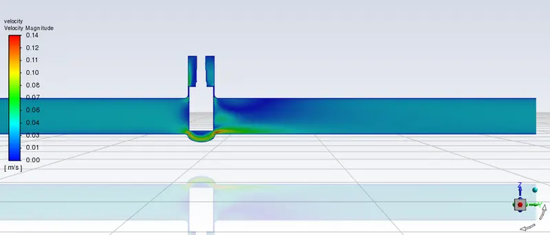
6) Velocity Contour
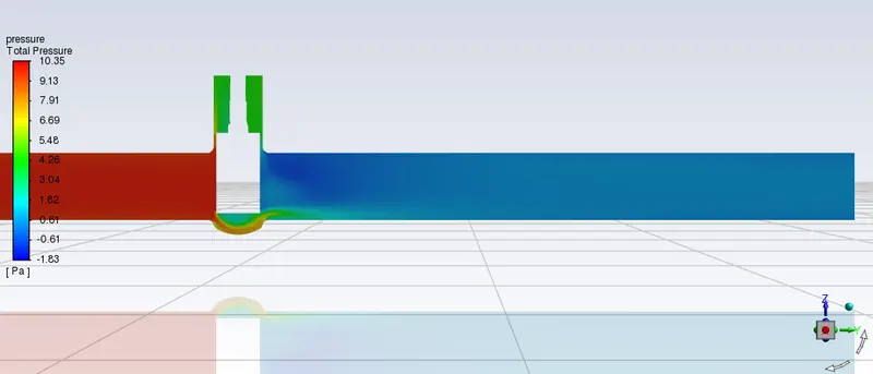
7) Pressure contour
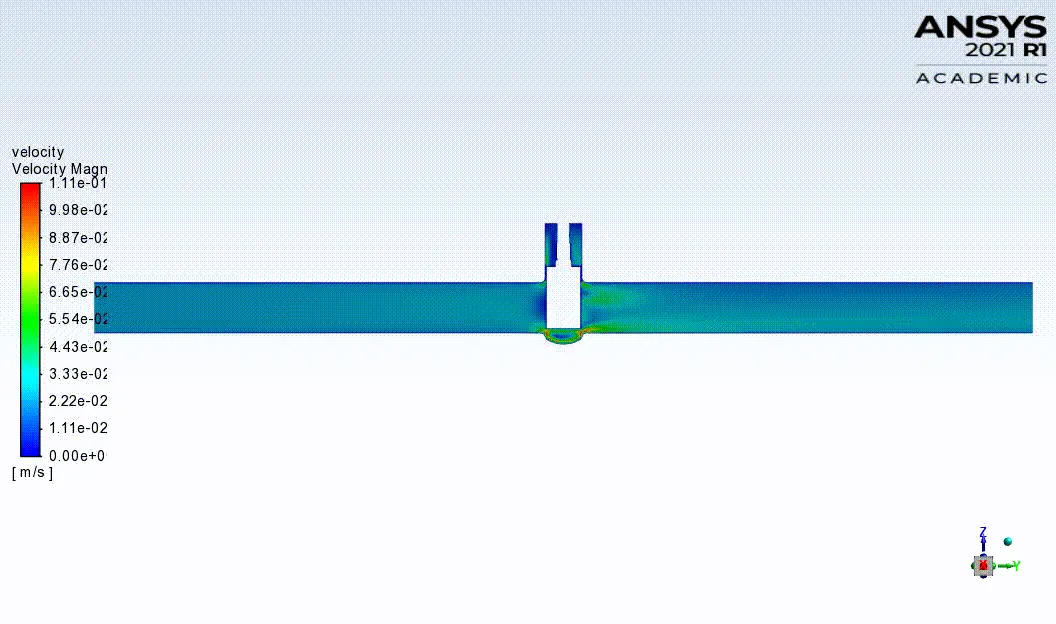
8) Animation of Velocity
Result – Lift 30mm
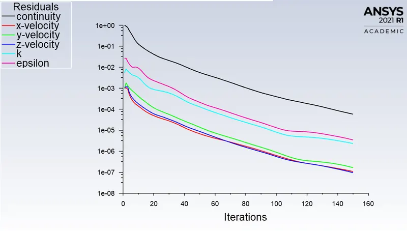
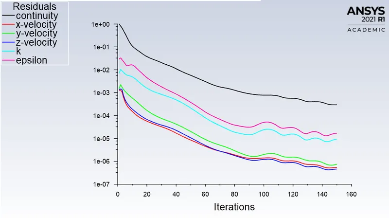
1) Residuals
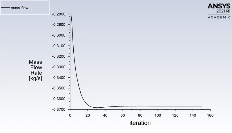
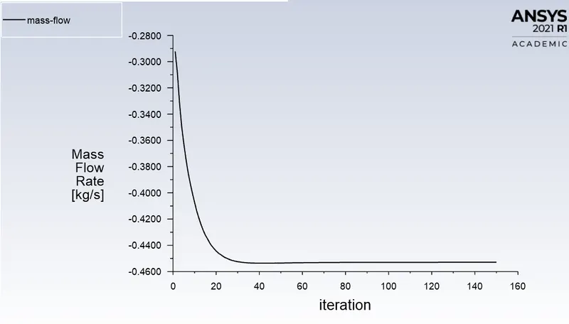
2) Mass flow rate
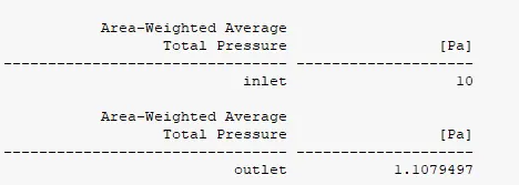
3) Pressure result
4) Flow Coefficient
Mass flow rate = 0.366 kg/s
Mass flow rate in US gallons per minute = 5.80 GPM
Inlet pressure in psi = 0.00145 psi
Outlet pressure in psi = 0.000160 psi
Pressure drop = Inlet pressure – Outlet pressure = 0.0012 psi
Specific gravity of water = 1 gm/cc.
`Cv=5.80√(1/0.0012)=167.43`
5) Flow Factor
Mass flow rate = 0.366 kg/s
Mass flow rate in m3/hr = 1.32 m3/hr
Inlet pressure in bar = 1e-4 bar
Outlet pressure in bar = 1.107-5 bar
Pressure drop = Inlet pressure – Outlet pressure = 0.000088 bar
Specific gravity of water = 1 gm/cc.
`Kv=1.32√(1/0.000088)=144.82`
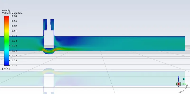
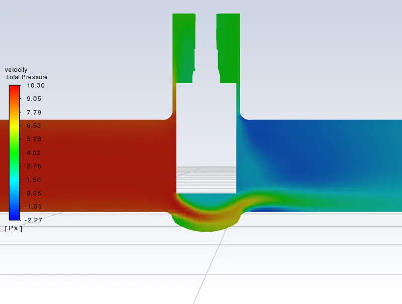
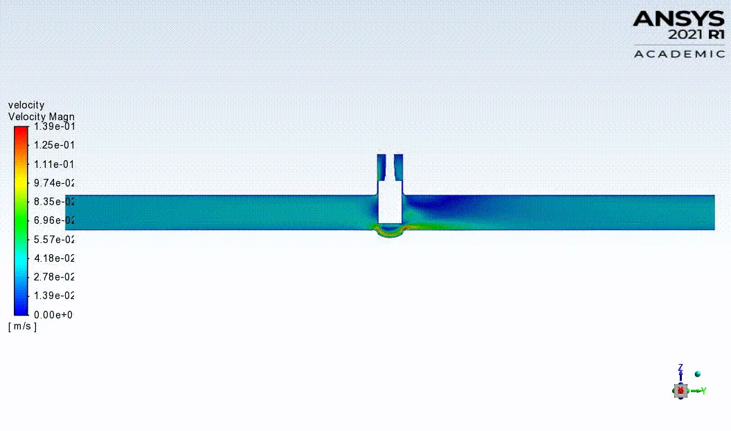
6) Velocity Contour
7) Pressure Contour
8) Animation of Velocity
Result – Lift 40mm
1) Residuals
2) Mass Flow Rate
3) Pressure Result
4) Flow Coefficient
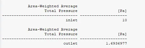
Mass flow rate = 0.452 kg/s
Mass flow rate in US gallons per minute = 7.16 GPM
Inlet pressure in psi = 0.00145 psi
Outlet pressure in psi = 0.000245 psi
Pressure drop = Inlet pressure – Outlet pressure = 0.001155 psi
Specific gravity of water = 1 gm/cc.
`Cv=7.16√(1/0.001155)=210.67`
5) Flow Factor
Mass flow rate = 0.366 kg/s
Mass flow rate in m3/hr = 1.63 m3/hr
Inlet pressure in bar = 1e-4 bar
Outlet pressure in bar = 1.693-5 bar
Pressure drop = Inlet pressure – Outlet pressure = 0.0000830 bar
Specific gravity of water = 1 gm/cc.
`Kv=1.63√(1/0.0000830)=182.22`
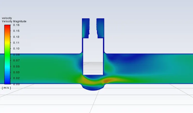
6) Velocity Contour
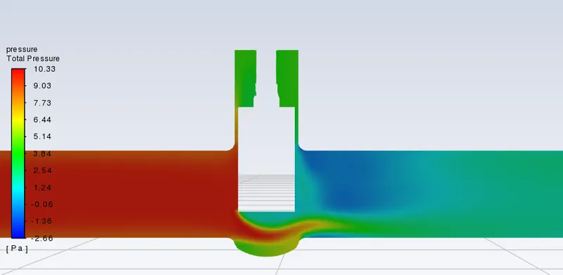
7) Pressure Contour
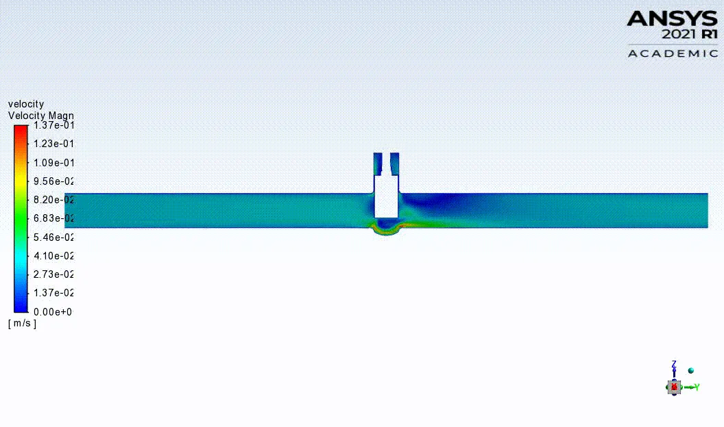
8) Animation of Velocity
Result – Lift 50mm
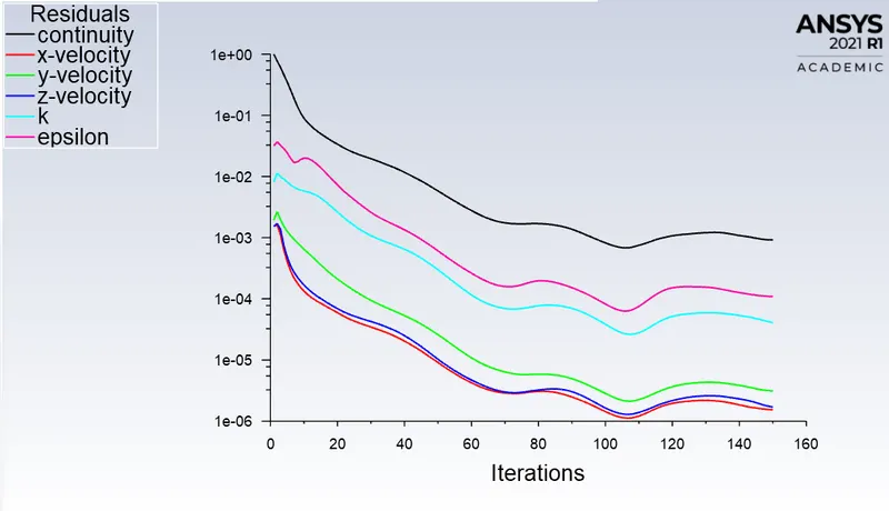
1) Residuals
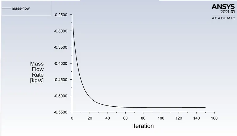
2) Mass flow rate
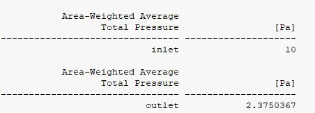
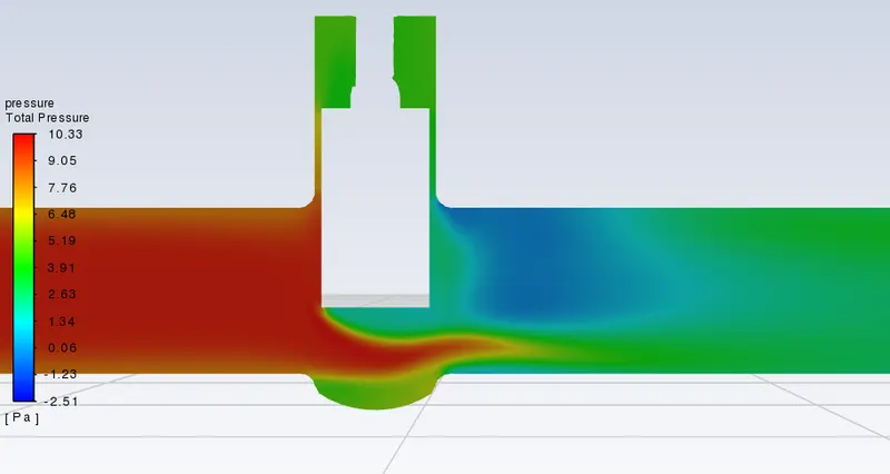
3) Pressure Result
4) Flow Coefficient
Mass flow rate = 0.535 kg/s
Mass flow rate in US gallons per minute = 8.48 GPM
Inlet pressure in psi = 0.00145 psi
Outlet pressure in psi = 0.000344 psi
Pressure drop = Inlet pressure – Outlet pressure = 0.0010556 psi
Specific gravity of water = 1 gm/cc.
`Cv=8.48√(1/0.001055)=266.95`
5) Flow Factor
Mass flow rate = 0.535 kg/s
Mass flow rate in m3/hr = 1.93 m3/hr
Inlet pressure in bar = 1e-4 bar
Outlet pressure in bar = 2.375-5 bar
Pressure drop = Inlet pressure – Outlet pressure = 0.0000762 bar
Specific gravity of water = 1 gm/cc.
`Kv=1.93√(1/0.0000762)=230.91`
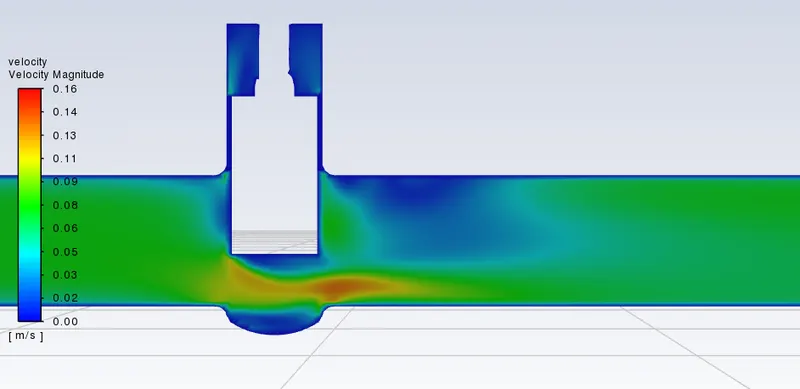
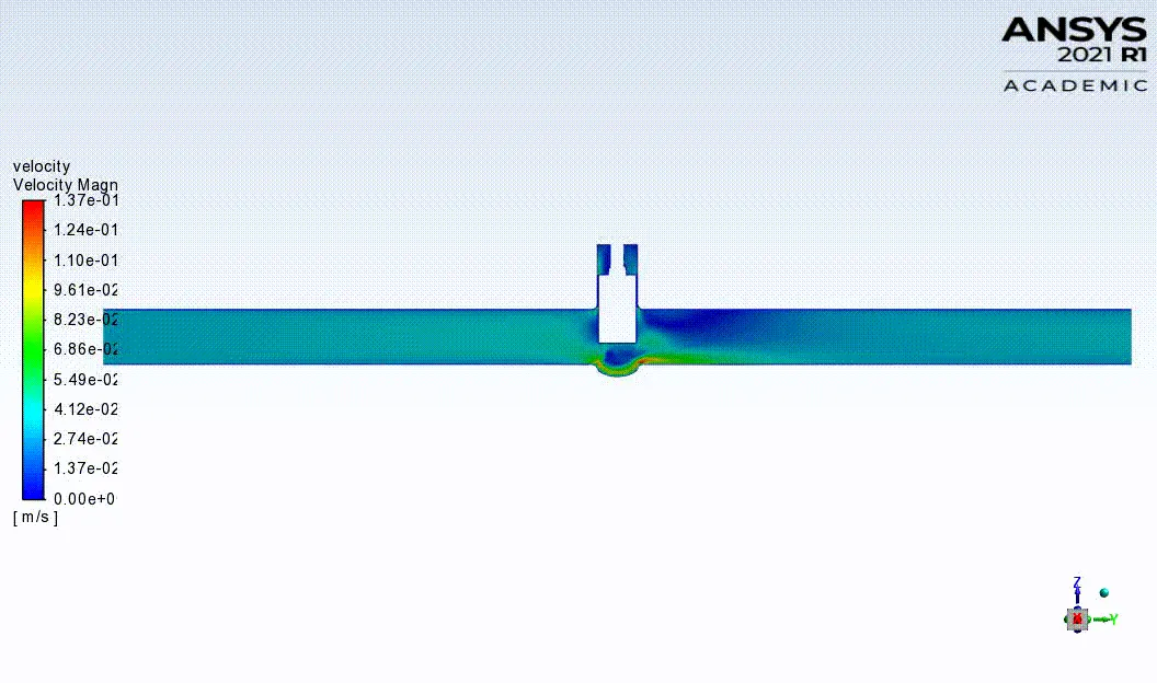
6) Velocity Contour
7) Pressure Contour
8) Animation of Velocity
Result – Lift 60mm
1)Residuals
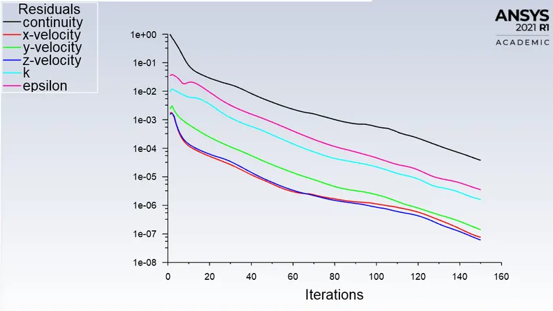
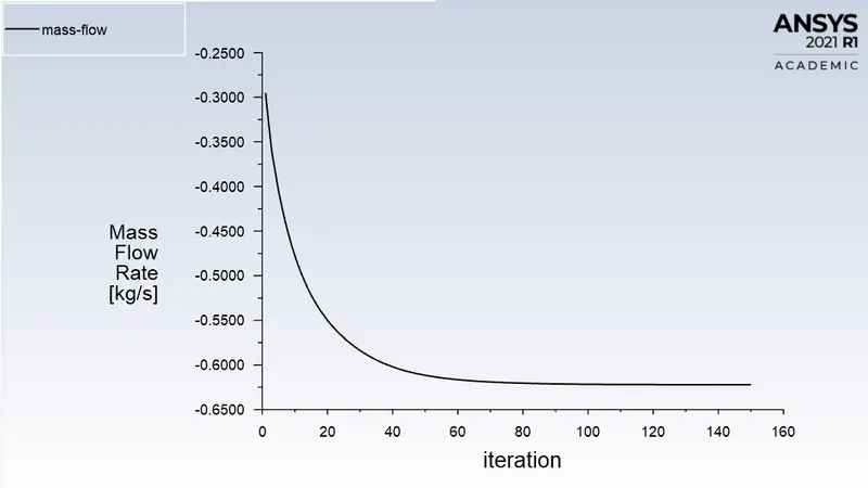
2) Mass flow rate
3) Pressure result
4) Flow Coefficient
Mass flow rate = 0.622 kg/s
Mass flow rate in US gallons per minute = 9.86 GPM
Inlet pressure in psi = 0.00145 psi
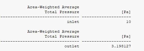
Outlet pressure in psi = 0.000463 psi
Pressure drop = Inlet pressure – Outlet pressure = 0.000937 psi
Specific gravity of water = 1 gm/cc.
`Cv=9.86√(1/0.000937)=322.122`
5) Flow Factor
Mass flow rate = 0.622 kg/s
Mass flow rate in m3/hr = 2.24 m3/hr
Inlet pressure in bar = 1e-4 bar
Outlet pressure in bar = 3.196-5 bar
Pressure drop = Inlet pressure – Outlet pressure = 0.0000680 bar
Specific gravity of water = 1 gm/cc.
`Kv=2.24√(1/0.0000680)=278.62`
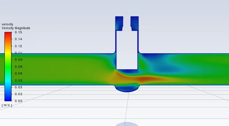
6) Velocity Contour
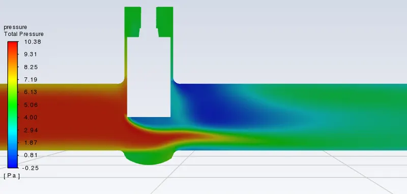
7) Pressure Contour
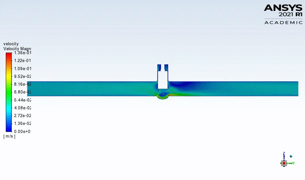
8) Animation of Velocity
Result – Lift 70mm
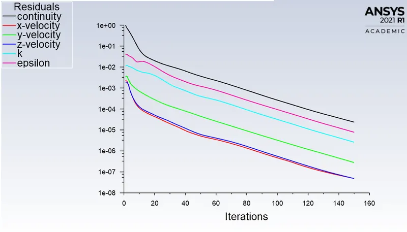
1) Residuals
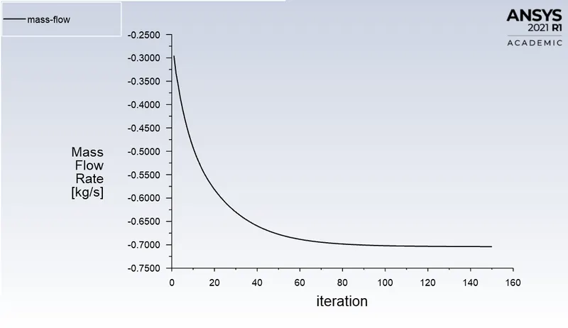
2) Mass flow rate
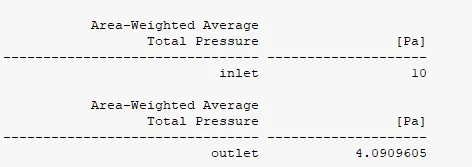
3) Pressure result
4) Flow Coefficient
Mass flow rate = 0.703 kg/s
Mass flow rate in US gallons per minute = 11.14 GPM
Inlet pressure in psi = 0.00145 psi
Outlet pressure in psi = 0.000593 psi
Pressure drop = Inlet pressure – Outlet pressure = 0.000807 psi
Specific gravity of water = 1 gm/cc.
`Cv=11.14√(1/0.000807)=392.146`
5) Flow Factor
Mass flow rate = 0.703 kg/s
Mass flow rate in m3/hr = 2.53 m3/hr
Inlet pressure in bar = 1e-4 bar
Outlet pressure in bar = 4.09-5 bar
Pressure drop = Inlet pressure – Outlet pressure = 0.0000591 bar
Specific gravity of water = 1 gm/cc.
`Kv=2.53√(1/0.0000591)=339.20`
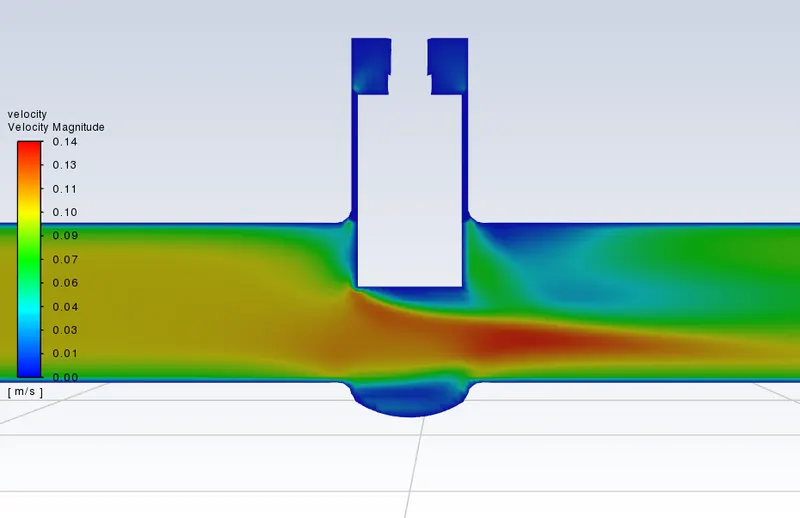
6) Velocity Contour
7) Pressure Contour
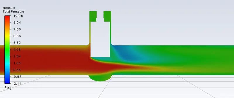
8) Animation of velocity
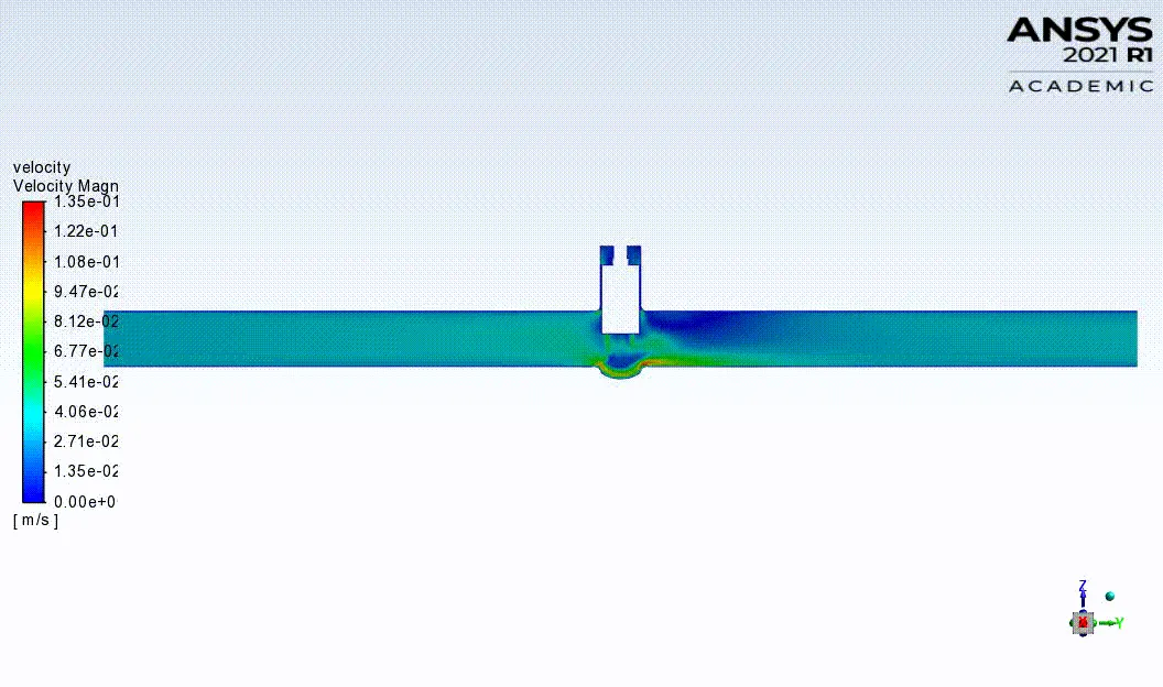
Result – Lift 80mm
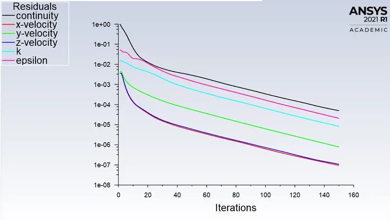
1) Residuals
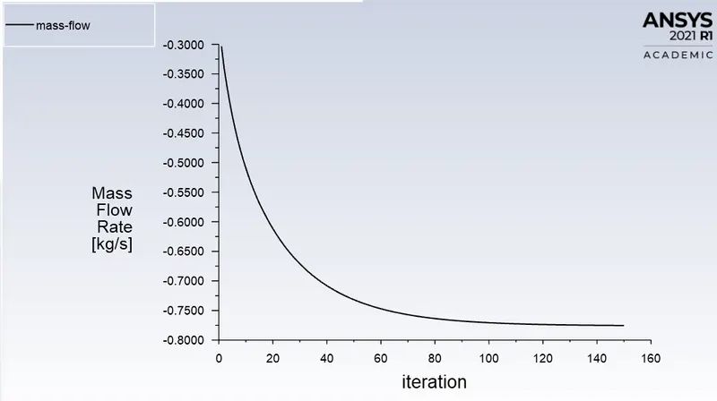
2) Mass flow rate
3) Pressure result
4) Flow Coefficient
Mass flow rate = 0.775 kg/s
Mass flow rate in US gallons per minute = 12.28 GPM
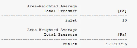
Inlet pressure in psi = 0.00145 psi
Outlet pressure in psi = 0.000721 psi
Pressure drop = Inlet pressure – Outlet pressure = 0.000679 psi
Specific gravity of water = 1 gm/cc.
`Cv=12.28√(1/0.000679)=471.26`
5) Flow Factor
Mass flow rate = 0.775 kg/s
Mass flow rate in m3/hr = 2.79 m3/hr
Inlet pressure in bar = 1e-4 bar
Outlet pressure in bar = 4.97-5 bar
Pressure drop = Inlet pressure – Outlet pressure = 0.00005026 bar
Specific gravity of water = 1 gm/cc.
`Kv=2.79√(1/0.00005026)=407.64`
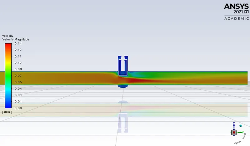
6) Velocity Contour
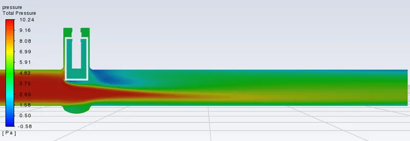
7) Pressure Contour
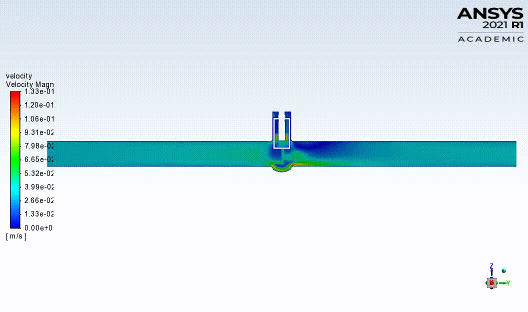
8) Animation of Velocity
Result – Lift 90mm
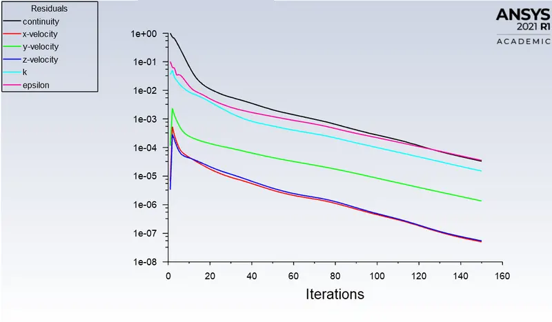
1) Residuals
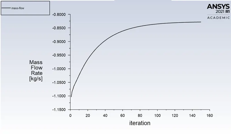
2) Mass Flow rate
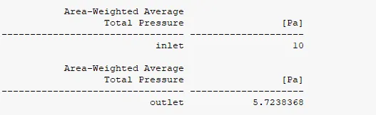
3) Pressure result
4) Flow Coefficient
Mass flow rate = 0.828 kg/s
Mass flow rate in US gallons per minute = 13.12 GPM
Inlet pressure in psi = 0.00145 psi
Outlet pressure in psi = 0.000830 psi
Pressure drop = Inlet pressure – Outlet pressure = 0.000570 psi
Specific gravity of water = 1 gm/cc.
`Cv=13.12√(1/0.000570)=549.536`
5) Flow Factor
Mass flow rate = 0.828 kg/s
Mass flow rate in m3/hr = 2.98 m3/hr
Inlet pressure in bar = 1e-4 bar
Outlet pressure in bar = 5.72-5 bar
Pressure drop = Inlet pressure – Outlet pressure = 0.00004277 bar
Specific gravity of water = 1 gm/cc.
`Kv=2.98√(1/0.00004277)=475.34`
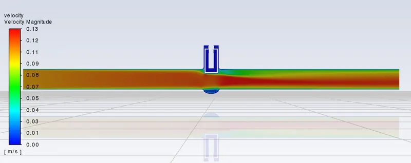
6) Velocity Contour
7) Pressure Contour
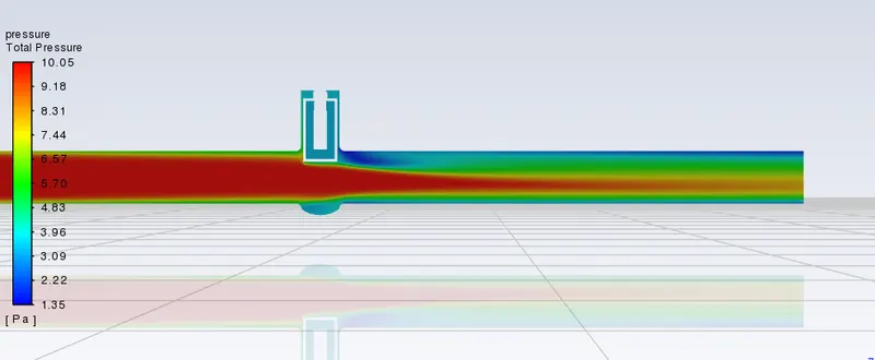
8) Animation of Velocity
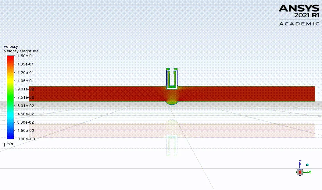
Parametric Results
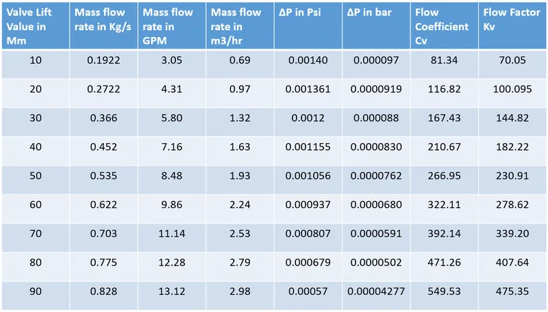
Result Table
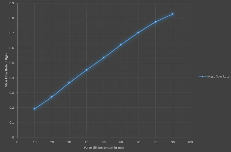
Result - Graph of Mass flow Rate with Valve Lift Increments
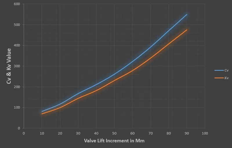
Result – Graph of Cv and Kv with Valve lift
Conclusion
1) From the all simulations it is evident that increase in lift will increase in mass flow rate fluid at outlet.
2) The increase of lift also have increment in the flow coefficient and flow factor i.e. Valve lift increment is directly proportional to Flow coefficient and flow factor.
3) From the graph of Lift increment and flow coefficient and flow factor, the line Cv and Kv are not in linear direction and we have low Kv for respective Cv depend upon the unit system.
4) As the valve get lifted the pressure at outside of the system is also increases and presssure difference is decreasing with each valve disc height increment.
5) The cartersian mesh provide better quality of result with respect to patch conforming mesh for the problem.
6) Parametric study helps to save time for each of case and retaining the data helps in acquiring the result as quick as possible for post-processing.