Week 5: Prandtl Meyer Shock problem
Week 5 – Prandtl Meyer Shock Problem
Aim: - Performing the Prandtl Meyer shock problem for subsonic and supersonic flow with adaptive mesh refinement.
Objectives: -
1) To study the importance of Prandtl Meyer Shock problem and its applications.
2) To study the types of boundary used for the simulations.
3) To study the importance of Neumann boundary conditions for shock problems.
4) To setup the simulation of 2D case geometry for supersonic flow with sharp angle.
5) To Change the sub-grid criterion for the simulation and check the results.
6) To perform the simulation for sub-sonic flow and compared with super-sonic flow phenomenon.
Introduction: -
When an object moves in the flow field of gas or any other fluid, it tries to deflect the molecules around the object. When such object is moving at much lesser speed than that of speed of sound, the density of the fluid remain constant and flow of the gas around the object can be determined by the conservation of mass and momentum. As the speed of the object is increased towards the speed of sound, the density of flow start to change locally as the gas is get compressed by the object. As the speed of object is more than the speed of sound, there is the abrupt decrease in the flow area and shock waves generated. If the flow speed of object increase beyond the speed of sound and the flow area is getting increase, then this phenomenon is called centered expansion fan.
There is some marked difference between this two phenomenon which are shock waves and centered expansion fan. In the shock wave phenomenon, the Mach number get decrease and the static pressure is increased and there is loss of total pressure because the process is totally irreversible in nature. Whereas the expansion process is isentropic in nature, in which the Mach number get increased and static pressure get decreased which result in total pressure constant in nature.
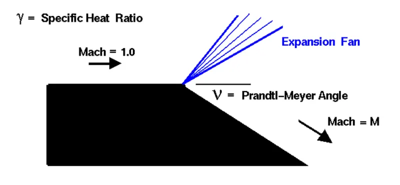
Calculation of the centered expansion fan involves the use of Prandtl Meyer Function. The function is derived from the same mass, momentum and energy phenomenon for very small differential deflections. The amount of increase in the Mach number is depend upon the inlet velocity and the angle of expansion. The interpretation of function is simply as; it is the angle through which you must expand a sonic flow to obtain a given Mach number.
Types of Boundary Conditions:
The CFD simulation of any problem consist of solving governing equation in the form of integral or differential form. This equation requires either initial condition or specified boundary conditions for solving of problem. Depending upon type of partial differential equation, number of boundary conditions are required. In case of super-sonic flow, the hyperbolic equations are used which have one characteristic line and one imaginary line hence it requires both initial condition at the inlet of domain and boundary conditions at the outlet of domain. The boundary condition which are required at the outlet are mostly Neumann condition which means the differential form. There are 5 types of boundary conditions which are mostly used in the simulation.
1) Dirichlet Boundary Condition
This type of boundary conditions is also called as initial boundary conditions. When this boundary condition is imposed on any partial differential equation, it will specify the value of solution which will take on the boundary.
2) Neumann Boundary Condition
This type of boundary condition is used when the condition at the domain are not specified. The value at the boundary is computed from the initial condition or the specified value provided at inlet. When imposed on the ordinary or partial differential equation, the condition specifies the value in which derivative of solution is applied within the domain.
3) Robin Boundary Condition
The Robin boundary condition consist of a linear combination of values of the field and its derivatives on the boundary. This boundary condition is also called as impedance boundary condition. In case of structural simulation this boundary condition is set to determine how much it resist to motion when harmonic load is applied. In case of fluid dynamic this boundary condition is used as semi-reflective wall which absorb waves partially. This condition is mostly used for the pressure-based approach and mostly used in acoustic applications.
4) Mixed Boundary Conditions
The mixed boundary condition consists of applying different type of boundary condition in different part of domain. It is need to be aware that, it should be applied on the whole boundary as the free boundary is always Neumann condition. It is different from Robin boundary condition as it consist of different type of boundary condition applied to the same region of the computational domain.
5) Cauchy Boundary Conditions
The Cauchy boundary condition is applied to both unknown field and its derivatives. It consists of one Dirichlet BC and Neumann BC.
Why to Use Neumann Boundary Condition for Super-sonic flow:
In case of super-sonic flow, the speed of body is more than speed of sound. Hence a front is developing as body moves through field. The zone of action creates in front of body and the zone of disturbance is way more behind. Hence the value at the zone of action can’t be determined. As the value of pressure, velocity and temperature are not available before the solving problem. To compute the value at the outlet it is necessary to derive the value from the inside of domain. As the Neumann boundary condition provide the derivative of specified value from the domain hence it is necessary to use this type of boundary conditions for the simulations.
Solution Methodology:
In this problem the 2D simulation of Prandtl Meyer shock is done. It is considering as steady state problem as the change of velocity and pressure are not monitoring with respect to time. The flow is considering as steady but the due to high velocity the and the Mach number is 2 for the super-sonic flow, density based approach is used. This approach helps to determine the changes in the density which further helps to determine the flow properties. For better resolution result near the expansion angle it is necessary to use the adaptive mesh refinement approach in the simulation. The simulation is running for 25000 cycles with average velocity and temperature monitor for convergence purpose. The simulation is done for 4 cases.
Case 1 – Inlet velocity = 680 m/s, Sub-grid Criterion = 0.01
Case 2 – Inlet Velocity = 680 m/s, Sub-grid Criterion = 0.05
Case 3 – Inlet Velocity = 680 m/s, Sub-grid Criterion = 0.1
Case 4 – Inlet Velocity = 100 m/s, Sub-grid Criterion = 0.05
This cases will be used to compare the result for different sub-grid criterion. Case 4 will be used to compare the result between the subsonic flow and supersonic flow.
Case Setup
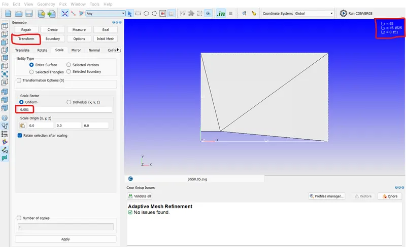
The geometry for the simulation is directly imported in the converge studio platform. It is necessary to check the dimension of model before beginning of simulation. The model is scaled to 0.001 factor to convert in meters.
1) Boundary Flagging
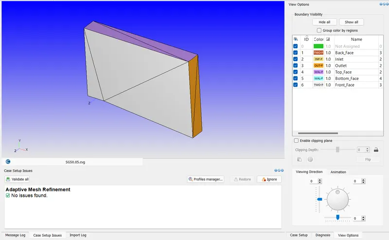
For the simulation in the converge studio it is important to create the boundaries. This boundary is treated as the input for the simulation. For this simulation inlet, outlet, top and bottom wall and front and back faces are created.
2) Solver Controls
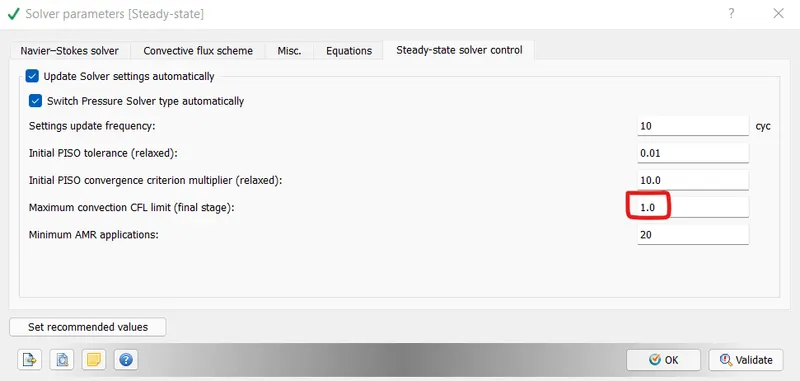
The case setup of this simulation is similar to previously done 2D simulation. The changes will be in the defining the solution parameters and the boundary conditions. In Run parameter the steady state solver has been choose with steady state monitors for monitoring convergence of simulation. The simulation time parameters are set to 25000 cycles with maximum time of 1 seconds. In the solution time parameter, it is necessary to confirm the maximum convection limit set to 1 for better convergence.
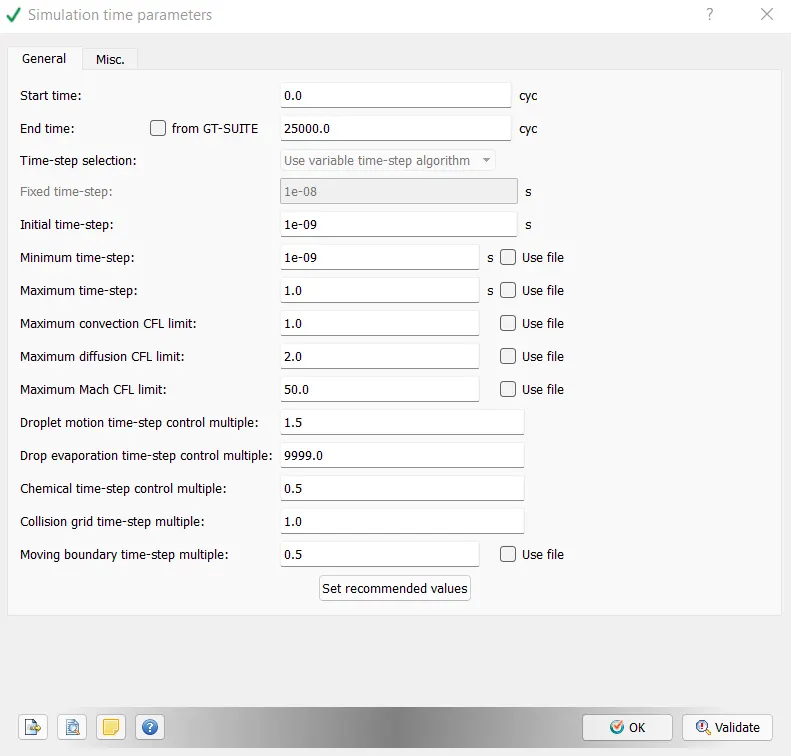
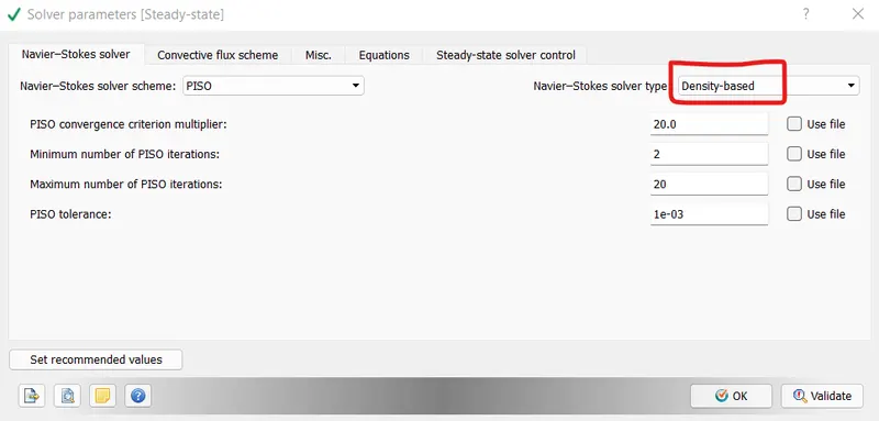
After setting up the solution parameter it is necessary to make sure the right solver has been selected. For this simulation as stated earlier density based approach has been used because of high Mach number. In the steady state solver control the maximum convection limit has to be set to 1 for better convergence purpose.
3) Initial & Boundary Conditions
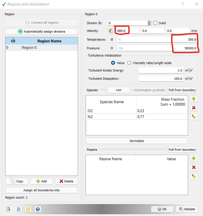
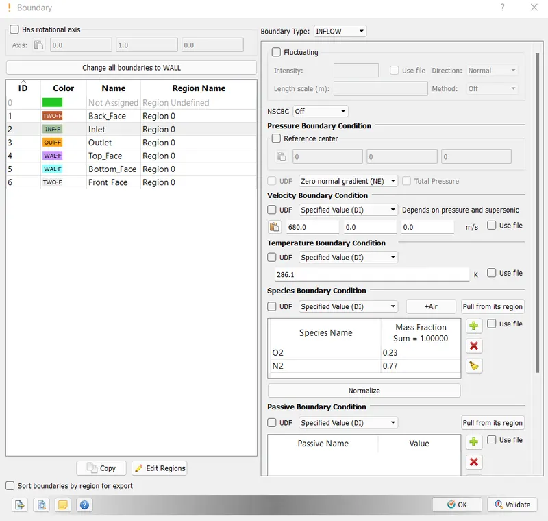
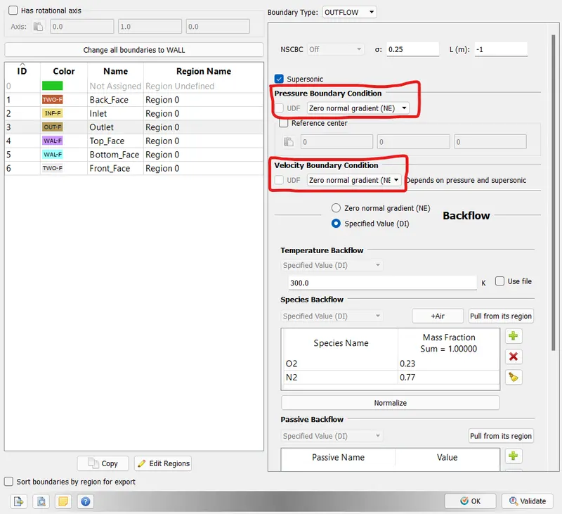
In case of supersonic flow condition, the initial conditions are treated as Dirichlet boundary condition which helps to derive the value of velocity, pressure and temperature at the outlet of domain using Neumann boundary conditions. For the initial condition it is necessary to provide the velocity of fluid inside the domain which is 680 m/s. The inlet pressure is 50000 Pascal’s with 300 kelvin of temperature.
A) Inlet Boundary Condition
B) Outlet Boundary Condition
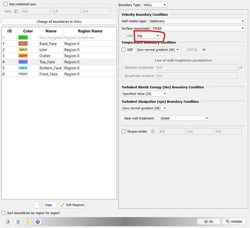
C) Wall Boundary Condition
4) Turbulence Model
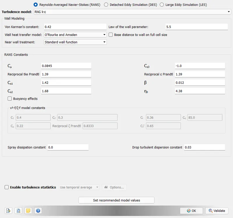
For this simulation as the flow speed is very high using RANS equation to calculate turbulence is bit of confusion. Because for high velocity flow the change in density cause the RANS equation to give unstable value. For most of high Mach number flows, LES equation is used to find the turbulence. In this case, the turbulence is not considering as an output variable hence RANS can be used for simulation also the simulation is in steady state approach. For this simulation RNG-K-epsilon model has been used.
5) Meshing
From the dimension of model, it can be seen that, it is bigger in dimension hence 0.8m size element in all direction are used for simulation.
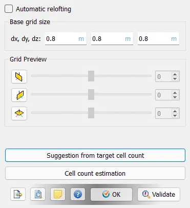
In Prandtl Meyer shock problem the region from the fist expansion line to the last line, the temperature and other parameter are changing rapidly. This is cause the solution to diverge if not enough element were present in the domain. Performing mesh intensive size simulation for whole domain again increase the time for problem also the load on the resources. This can be efficiently done by using the adaptive mesh refinement which is use the refinement zone depending upon the changes in the parameter. For adaptive mesh refinement, it is necessary to select which parameter has been changing rapidly with flow.
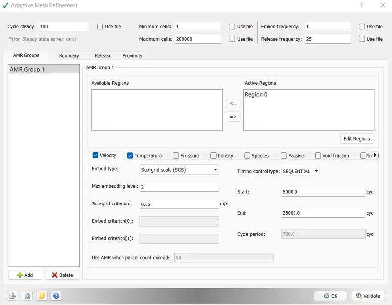
The rest of the setup is kept similar to other simulation the only difference is to create the 3D output data after every 100 cycles.
After exporting the input files to the specific folder, Cygwin application has to be launch to run the simulation in which ‘mpiexec.exe –n 4 converge.exe restricted’ command is used to start the simulation. The simulation takes 15688 cycles to converge which gives almost 156 files to read the data for post processing.
Result
Case 1 - Velocity = 680 m/s, Sub-grid Criterion = 0.01
1) Meshing before AMR
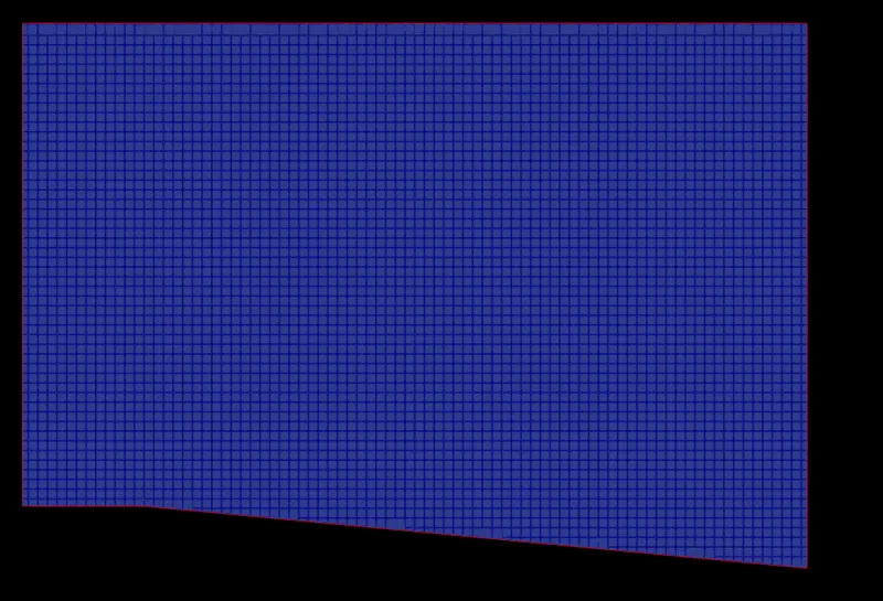
2) Meshing During AMR
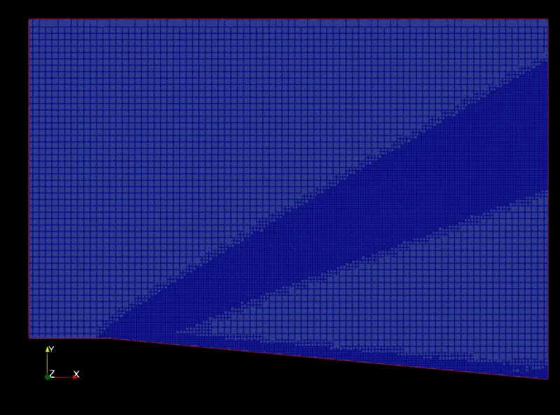
3) Density Contour
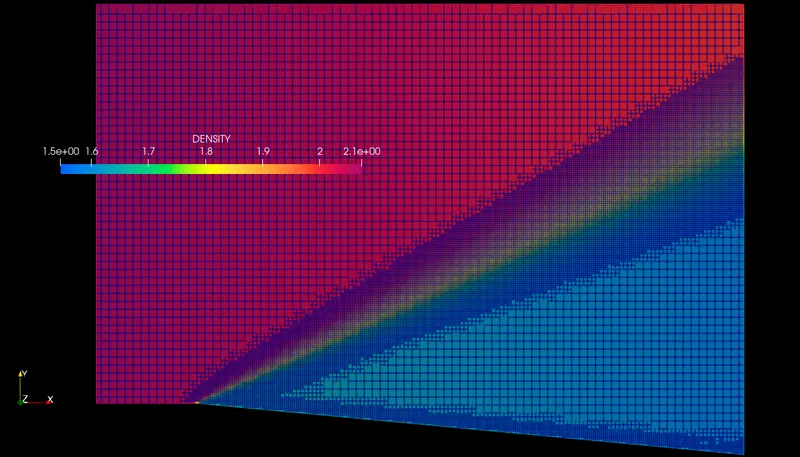
4) Pressure Contour
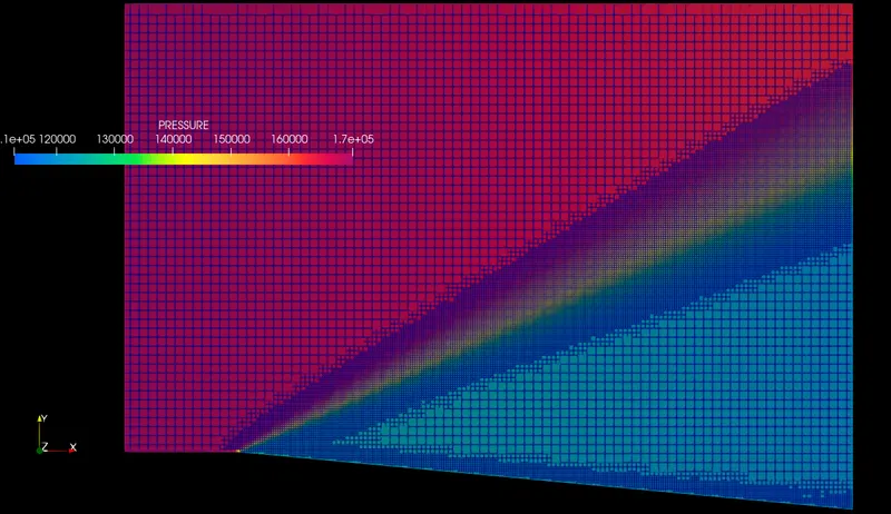
5) Velocity Contour
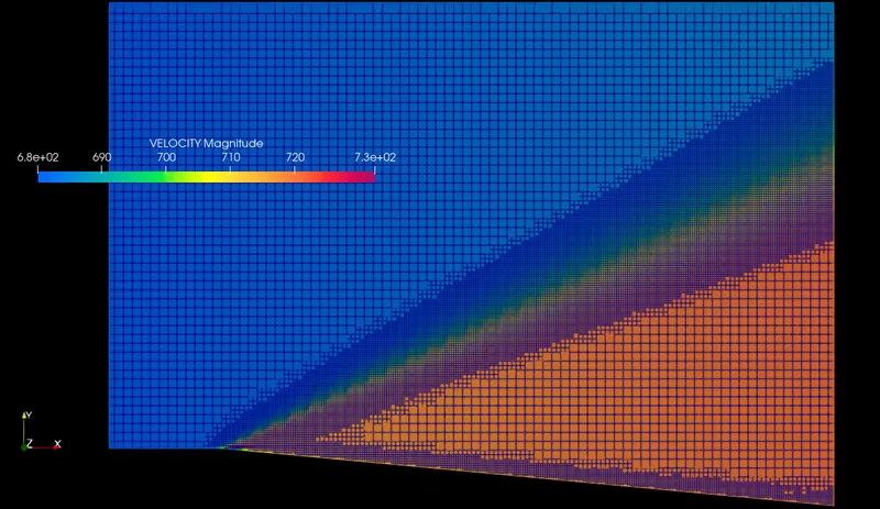
6) Temperature Contour
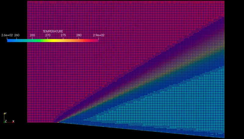
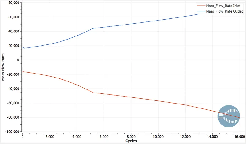
7) Mass flow rate plot
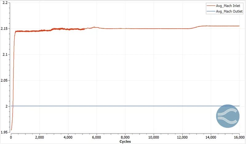
8) Mach Number Plot
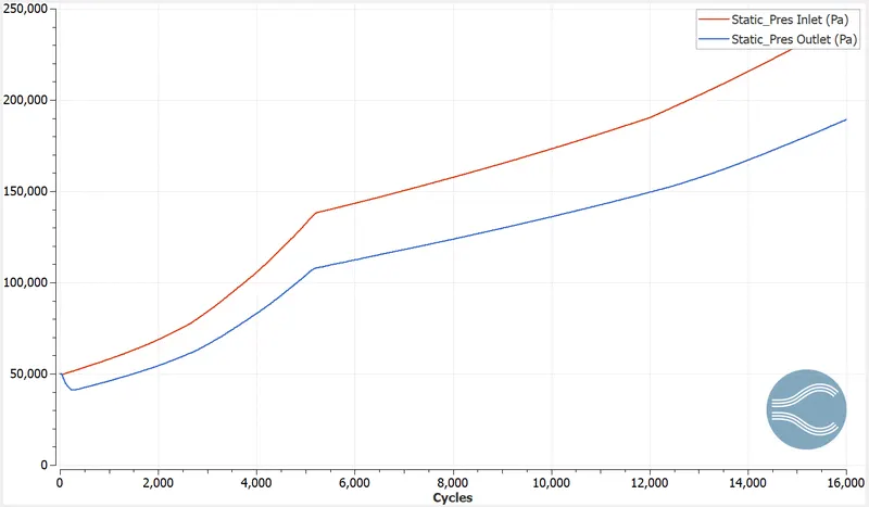
9) Static Pressure plot
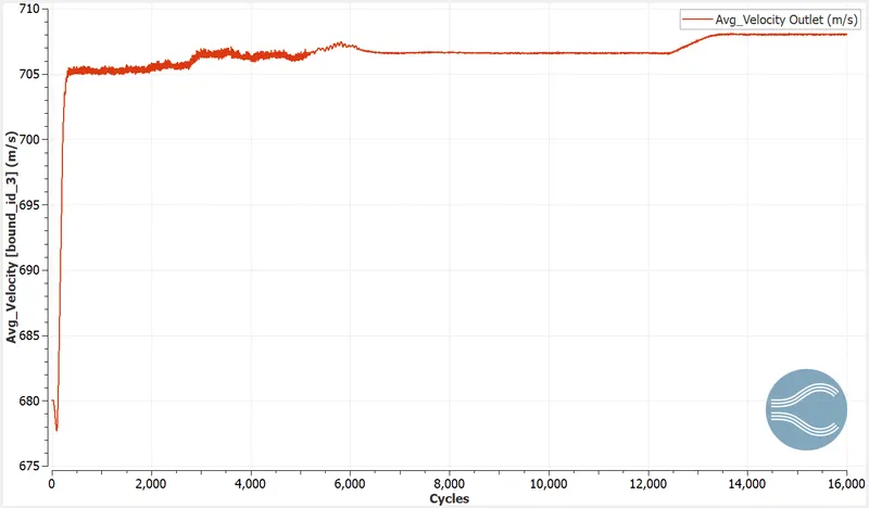
10) Avg Velocity Plot at Outlet
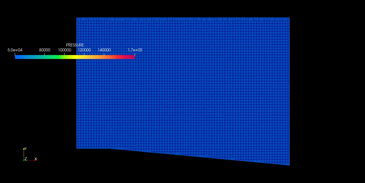
11) Pressure Animation
12) Density Animation
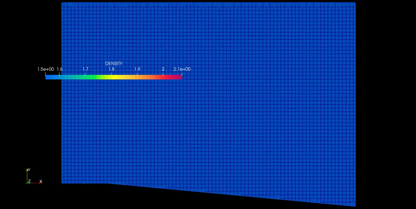
13) Velocity Contour Video
14) Pressure Contour Video
15) Temperature Contour Video
Case 2 - Velocity = 680 m/s, Sub-grid Criterion = 0.05
1) Grid Mesh before AMR
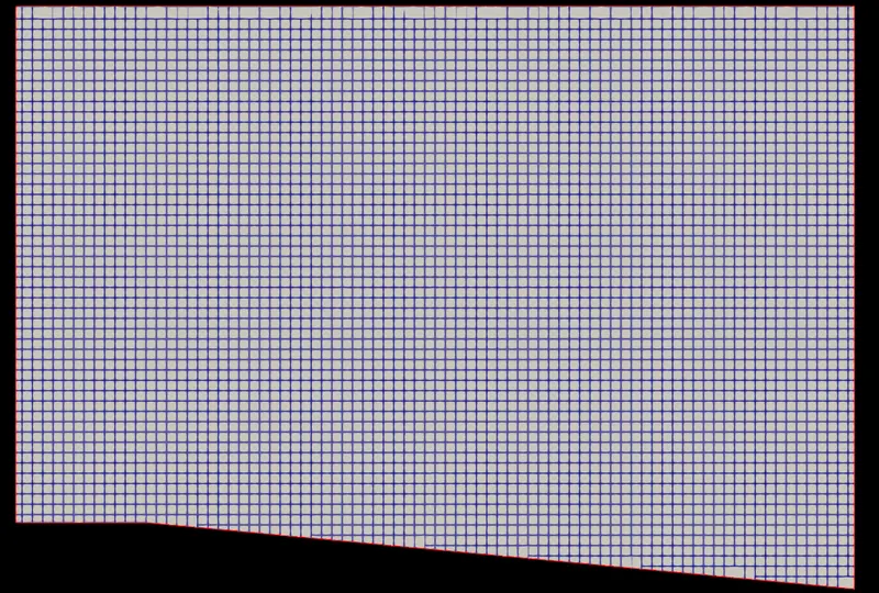
2) Grid Mesh after AMR
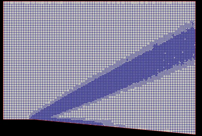
3) Velocity Contour
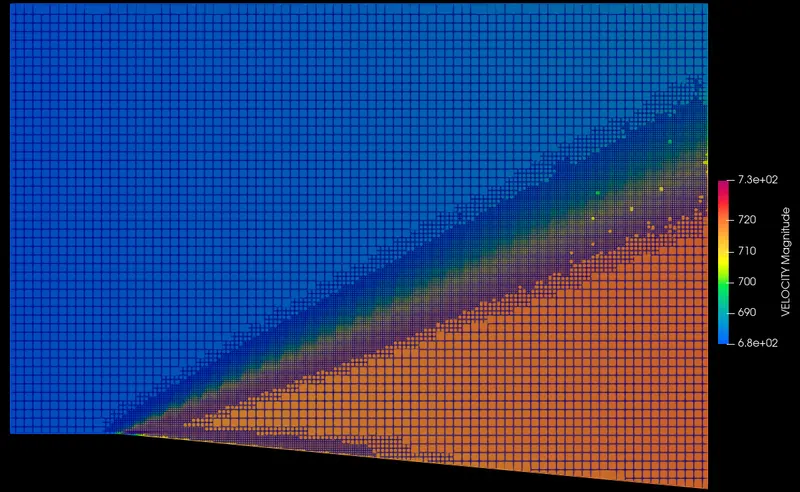
4) Pressure Contour
5) Temperature Contour
6) Density Contour
7) Static Pressure Plot
8) Mass flow rate plot
9) Mach Number Plot
10) Pressure Contour Animation
11) Denisty Contour Animation
12) Pressure Contour Video
13) Velocity Contour Video
14) Tempeature Contour Video
Case 3 - Velocity = 680 m/s, Sub-grid Criterion = 0.1
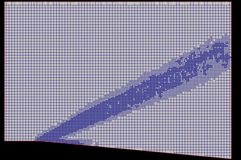
1) Grid After AMR
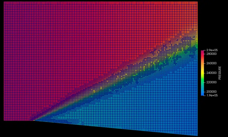
2) Pressure Contour
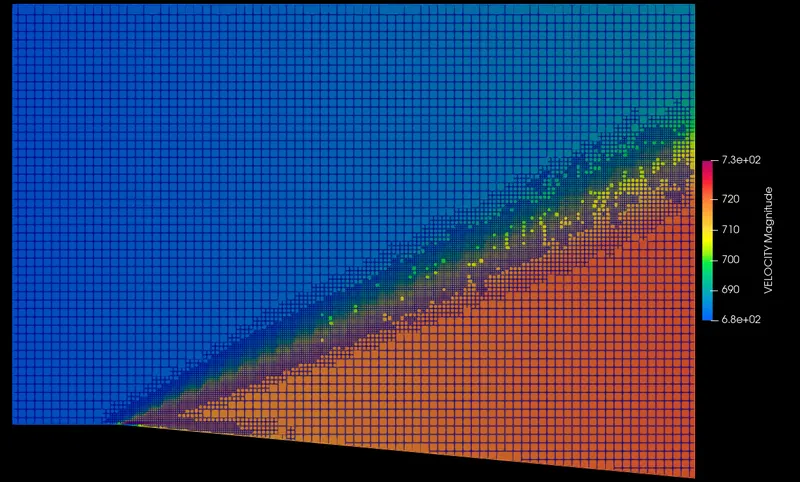
3) Velocity Contour
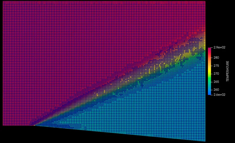
4) Temperature Contour
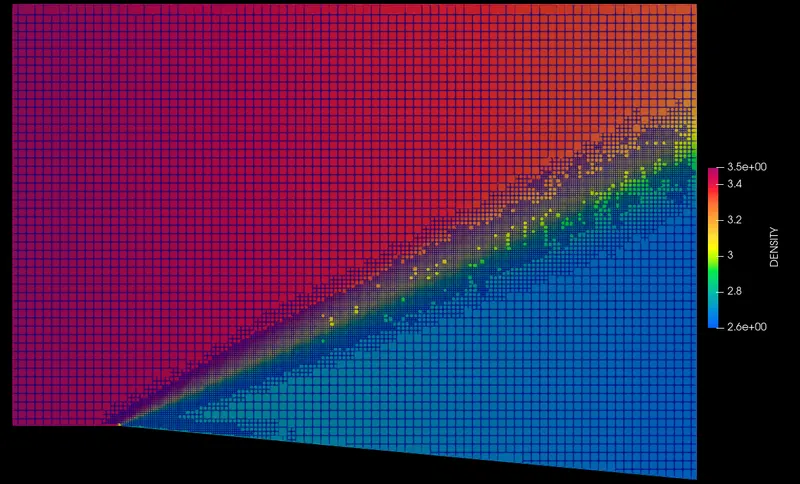
5) Density Contour
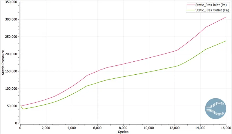
6) Static Pressure Plot
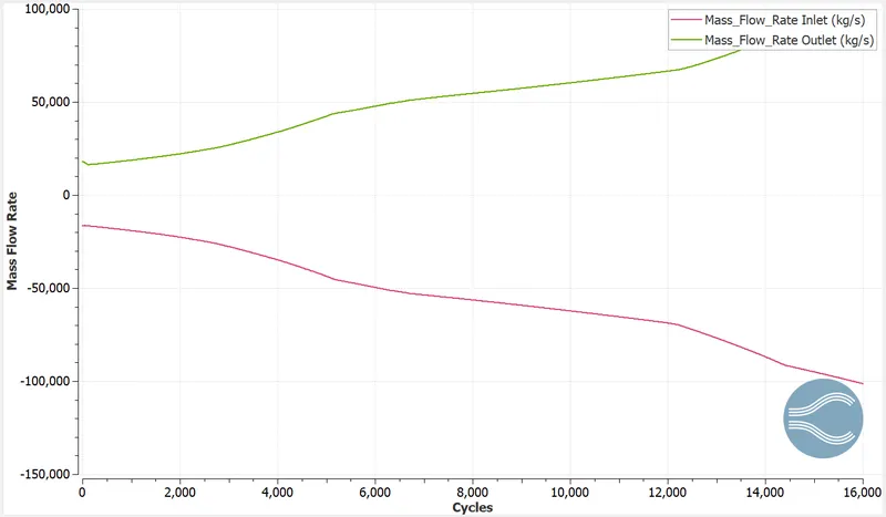
7) Mass flow Rate plot
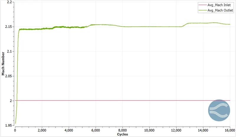
8) Mach Number Plot
9) Density Contour Animation
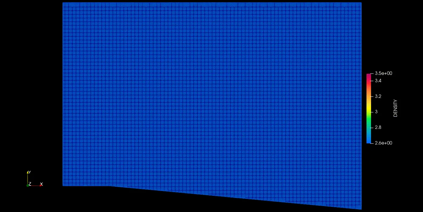
10) Pressure Animation
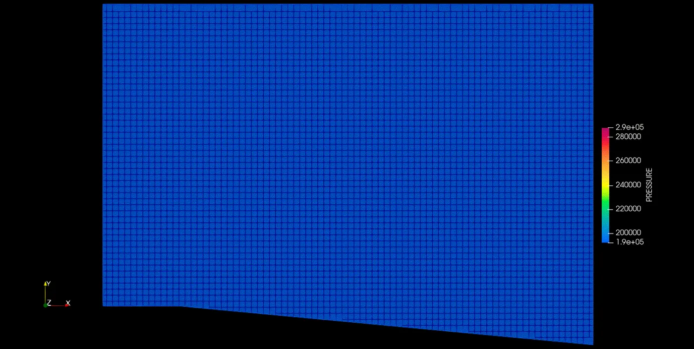
11) Velocity Contour Video
12) Pressure Contour Video
13) Temperature Contour
Case 4 - Velocity = 100 m/s, Sub-grid Criterion = 0.05 - Sub-Sonic Simulation
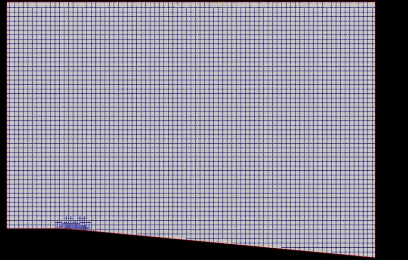
1) Grid Mesh
2) Pressure Contour
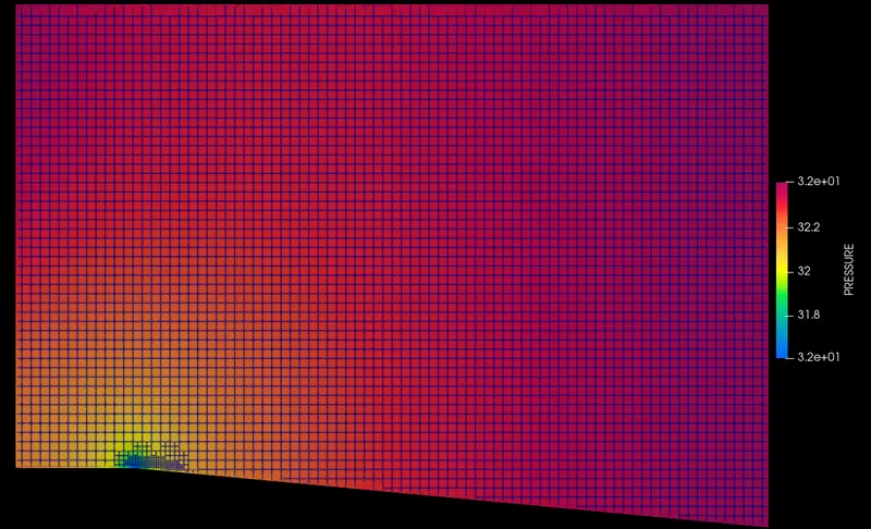
3) Velocity Contour
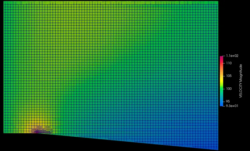
4) Temperature Contour
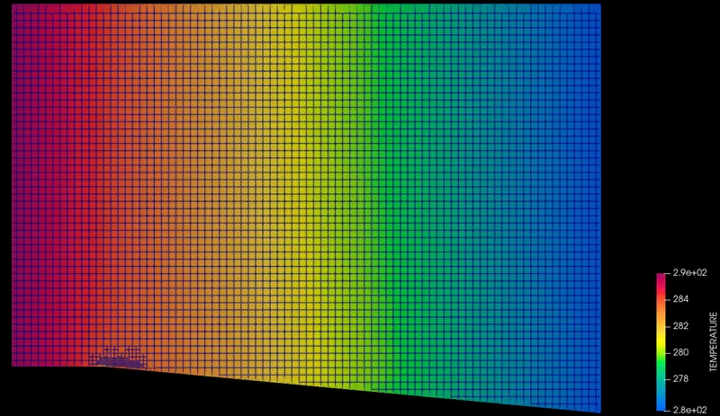
5) Density Contour
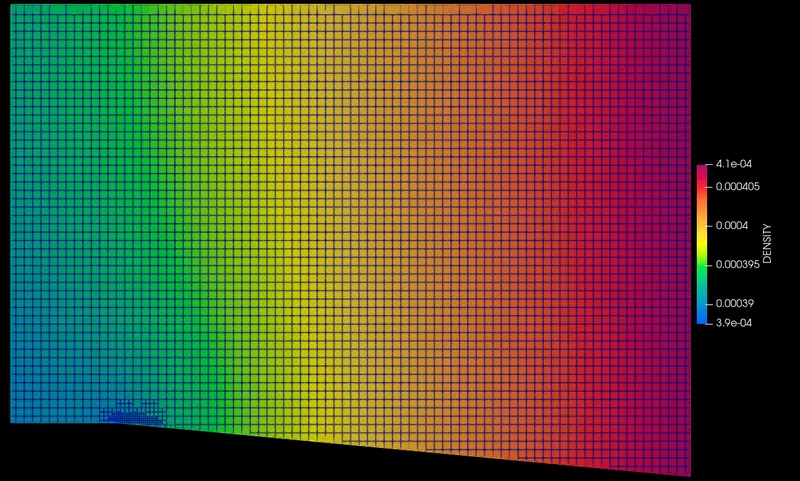
6) Static Pressure Plot
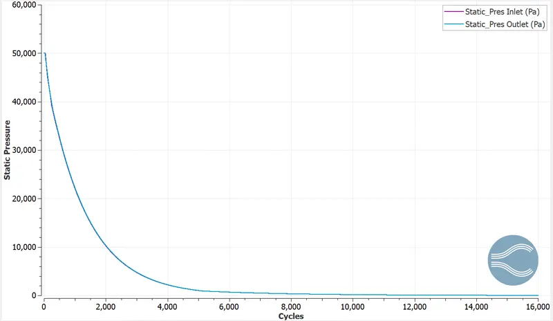
7) Mass flow rate Plot
8) Mach Number Plot
10) Density Animation
11) Pressure Contour Video
12) Velocity Contour Video
Observations
A) Effect of SGS
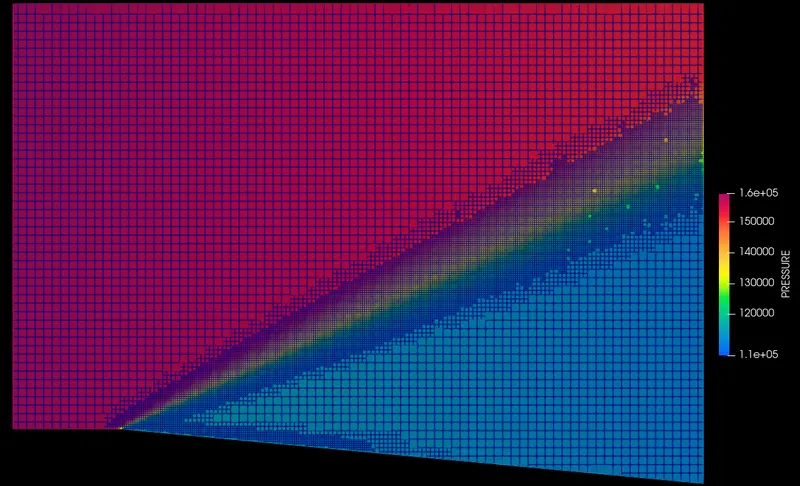
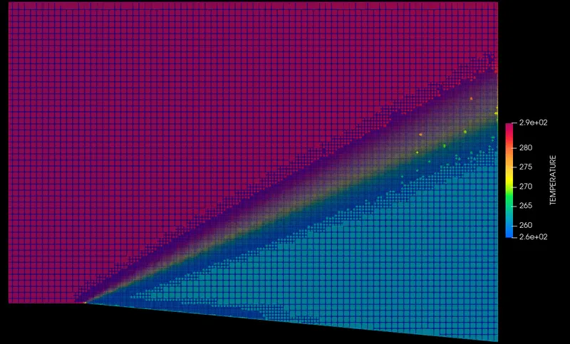
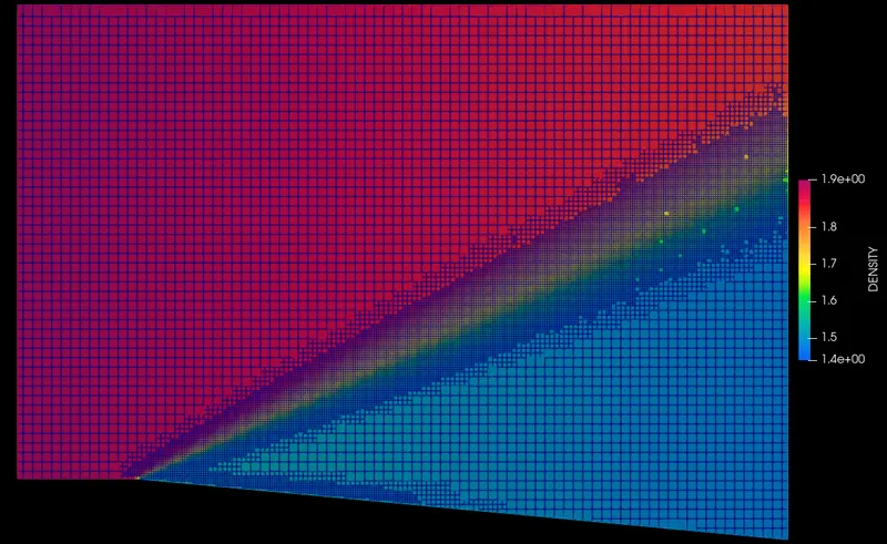
1) From the contour of different AMR with different sub-grid criterion it can be seen that decrease in number cause the increase in refinement over the greater area.
2) In case of SGS of 0.1 it can be seen that expansion fan angle is drastically reduced which means most of the parameter are not getting captured due to higher number criterion.
3) In this case of simulation, velocity and temperature both are used for refinement criteria. It can be seen that at the lower edge there is some refinement is done which is for velocity. As for simulation, turbulence model has been used hence near the boundary there is major changes in the velocity is happening which need to be captured during the flow.
B) Super-Sonic Vs Sub-Sonic
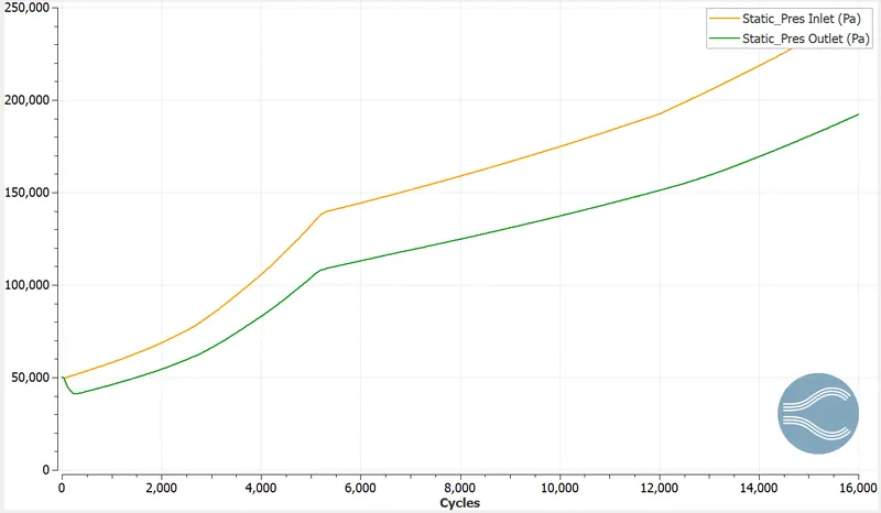
1) From case number 1 to 3 all the simulation were super-sonic in nature as the inlet velocity is more than speed of sound. In case number 4 the inlet velocity is 100 m/s which is lower than speed of sound. From the plot of static pressure, it can be seen that in case of super sonic flow the static pressure increase becasue of expansion fan phenomenon in which Mach number has to be increase fron the expansion zone. Where as in case of sub-sonic flow the static pressure is decreasing drastically due to creation of shock which lower the Mach number of flow.
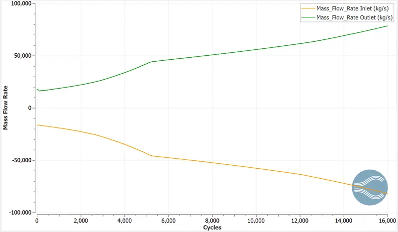
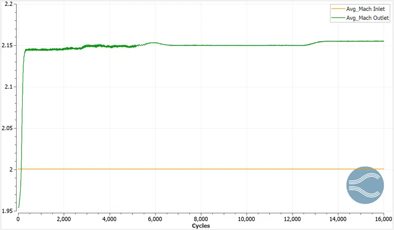
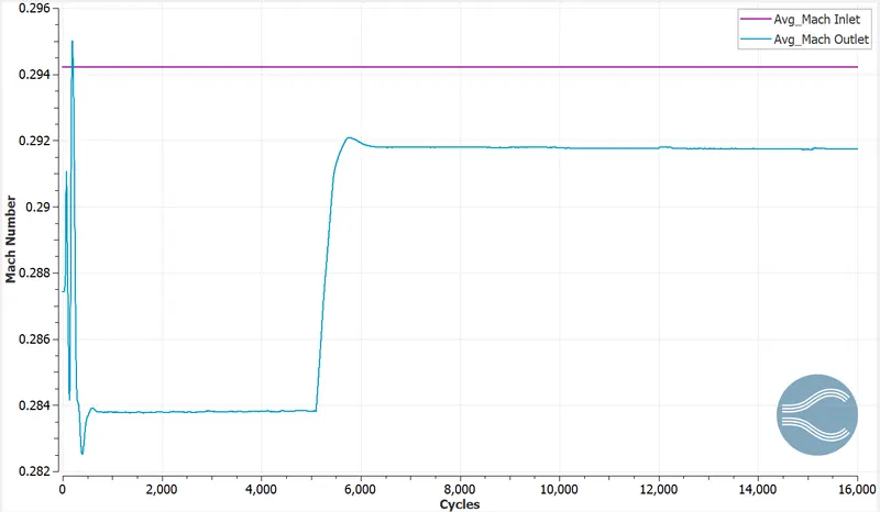
2) In case of sub sonic flow the Mach number at the outlet is lower than the inlet whereas in case of super-sonic the Mach number is increased to 2.15 compared to 2 at the inlet.
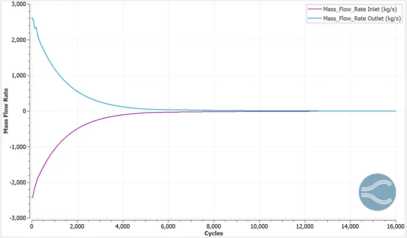
3) In case of Super sonic flow the mass flow rate at inlet and outlet obeys the mass conservation similar to subsonic flow but the difference is that, in sub-sonic flow the flow rate comes to zero after convergence telling flow is constant at both end.