Week 1- Mixing Tee
Aim: - Fluid flow simulation of Mixing Tee with different turbulence methods.
Objective: -
1) To study the initializing in ANSYS FLUENT for the project work.
2) To import the geometry in space-claim and pre-process for simulation.
3) To mesh the geometry with inflation layer and perform the steady state simulation for different cases.
4) To check convergence of solution and perform mesh indepentent test.
5) Use of parametrization for lowering the effort for each simulation process.
6) To discuss the effect of length and momentum ratio on simualtion results.
7) To post-process the result in convenient and explanable way.
Introduction: -
The project aims to produce the results which involve mixing of air at different temperature as well as different velocity in a mixing tee. The mixing tee are most use at the HVAC system were specific temperature is required. This mixing Tee are also used in low viscosity mixing systems also blending of oils. The effectiveness of this mixing tee is one of the important parameter which need to be discuss. The effectiveness involves providing specific velocity at inlets to get the desired result at outlet. The result which is required at the outlet can be a specific temperature or velocity of fluid.
This project involves to get the specific temperature at the outlet. The project is steady state simulation with different momentum ratio which determine the inlet velocity from the cold end of mixing tee. For better mixing it required turbulence, this has to be depend upon on the Reynolds number of fluid flow whether to go for turbulence model or not.
This simulation is setup in two different cases in which:
Case 1: - Short mixing tee with momentum ratio of 2 and 4 with K-espilon or K-omega SST model.
Case 2: - Long mixing tee with momentum ratio of 2 and 4 with turbulence model selected from the effectiveness of short mixing tee.
Approach toward the simulation: -
As simulation is steady state it does not required any time parameter to compute with. The simulation approach will start from the geometry clean-up and then towards the meshing. In meshing we will use the inflation layer to capture the boundary motion. As capturing the boundary motion is not required but it is good practice to provide inflation layer for internal flow simulation to get the desired result at end. For case 1 with inlet velocity at hot inlet is 3 m/s for short Tee application, we will use both K-espilon and K-omega SST turbulence model for each momentum ratio. From this we can determine which turbulence model is providing better results at the outlet. After that selected turbulence model will be used for Case 2 simulation where we are simulating long Tee with different momentum ratio. In the end we will study the mesh independent test by varying the size of mesh and see how much results are changes.
Pre-processing: -
- Geometry Clean-up
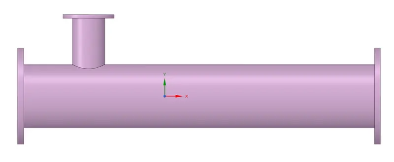
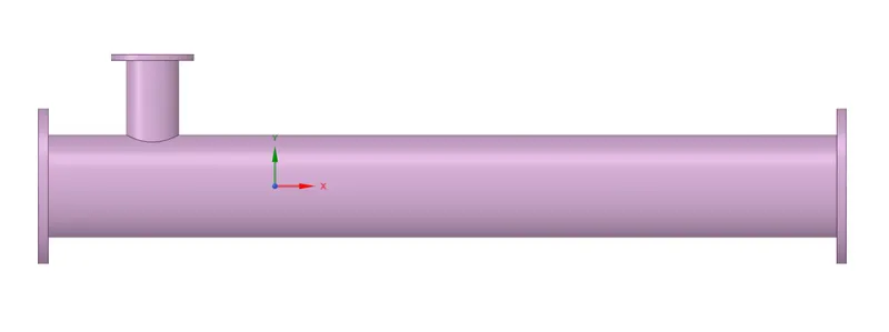
The pre-processing involves geometry clean-up, meshing, setting up boundary conditions. The geometry which are provided for simulation are:
- Short Mixing Tee
- Long Mixing Tee
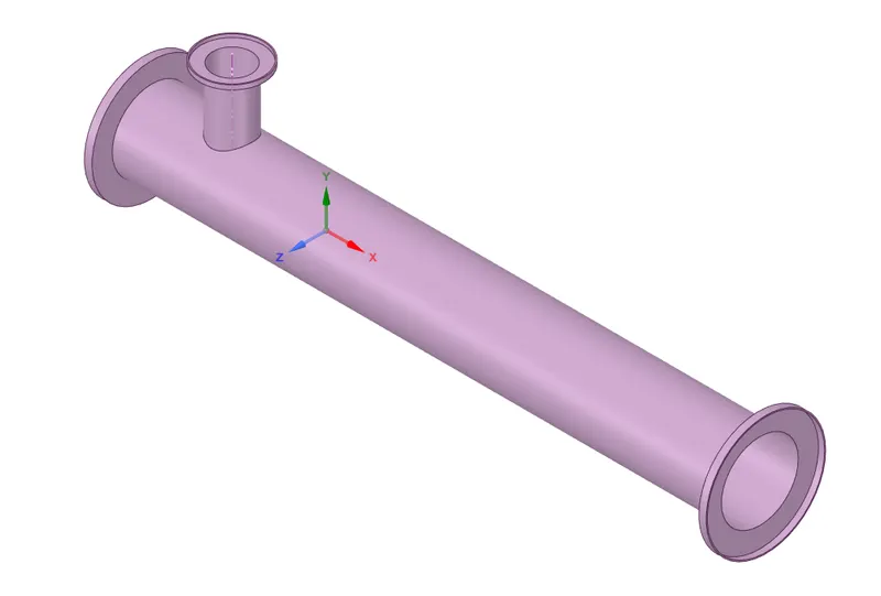
If we see the geometry from isometric view which is shown below, it has only outer section with inside section is hollow for fluid flow. It is important to create the fluid domain inside the geometry.
The fluid domain can be created by using prepare section of space-claim pre-processor. The tool which is used to create the fluid domain is volume extract in which we will use edge volume extraction. In this tool we will select the outer edges loops of geometry which resemble the fluid volume. This can be seen as:
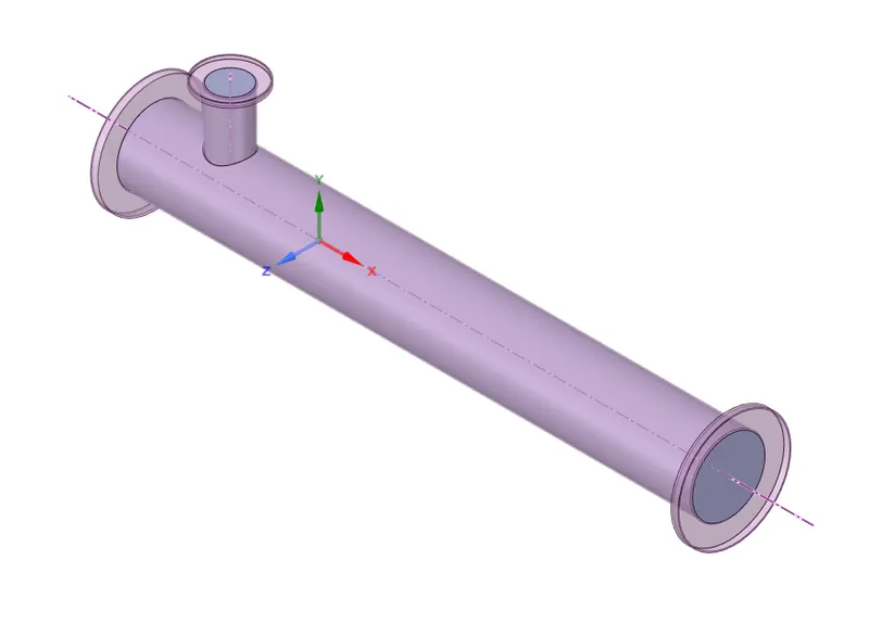
In above figure we can see grey color as fluid volume extracted using volume extraction tool and pink color shows the outer Tee section.
The extracted volume is the only requirement of the simulation as it is an internal flow simulation. Hence outer geometry can be supressed for simulation. After supressing the geometry, it will look like:
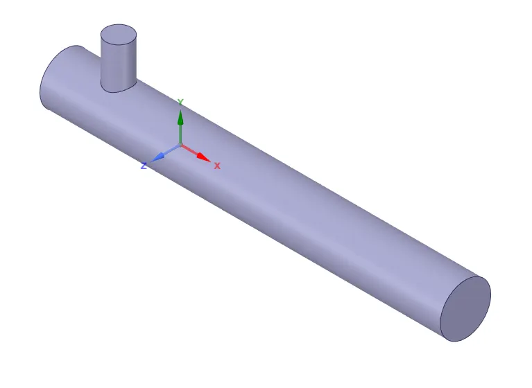
2.Meshing
After clean-up of geometry for simulation it is important to create mesh which is a volume mesh for fluid flow simulation. Creation of mesh gives the point at which governing equation to be solved. Finer the mesh will take more time for simulation hence it is necessary to provide required mesh size for the convenient simulation.
ANSYS workbench create mesh depend upon the physics we are solving. The physics preference we select should be CFD in which solver preference should be Fluent only. If we are using other solver like CFX or polyflow, the mesh preference should change accordingly. As most of meshing algorithm are already decided in ANSYS workbench it will create less fatigue for user while performing mesh.
The baseline mesh size selects for the both geometry is of 5mm and after performing baseline simulation for both turbulences model we will do the mesh independent test accordingly. ANSYS workbench takes care for the sizing function autonomously depend upon geometry features. In older version of ANSYS workbench sizing function can be selected by user. Sizing function provide more freedom over meshing platform. We are also using only linear element which is 1st order element for simulation. After providing mesh size of 5mm the geometry will look like:
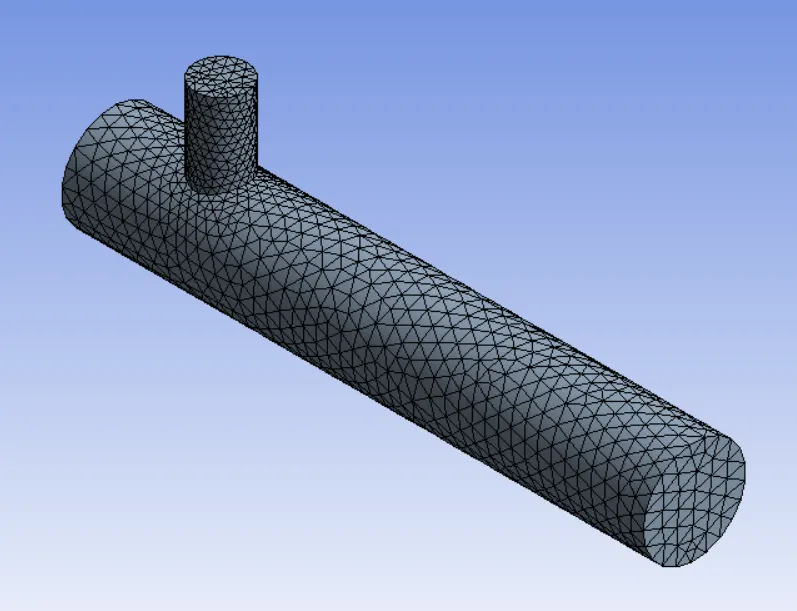
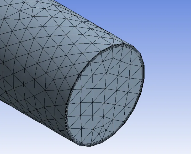
Creation of inflation layer will add better benefits to the simulation to capture the boundary layer motion. This can be added as local control of meshing in ANSYS workbench. The meshing control of ANSYS workbench are divided in two domains one is global control and other one is local control. Global control is meant to mesh whole geometry without taking care of most feature of geometry but local control can be used in accordance with global control to provide more meshing feature over the geometry. After providing inflation layer using option first layer thickness of 1mm and growth rate of 1.2 the mesh will look like:
Quality of mesh is one of the important thing in meshing. If the quality of mesh is way to worse, we can’t get the desired result from simulation or it will diverge the results from accurate results. In ANSYS workbench there are many quality criteria need to be studied but the most used quality criteria are skewness and orthogonal quality for fluid flow simulation. The skewness and the orthogonal quality are angle criteria of mesh element other than that jacobian and aspect ratio are length parameter of elements. The skewness criteria of mesh in mesh metric can be seen as:
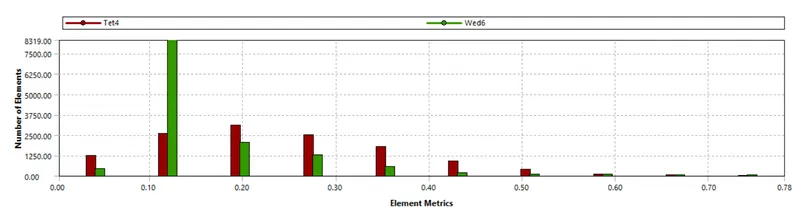
In this mesh metric we can see number element and mesh metric with what kind of elements are used in the mesh. Tet4 and wed6 are linear element and in skewness quality near to zero are best element and quality near to 1 are the worst element. Quality of element upto 0.95 are preferable for simulation.
3. Named Selection.
For any fluid flow simulation, it is important to provide the boundary condition with named selection from ANSYS workbench. ANSYS fluent require flow condition to simulate the problem which are initial condition and boundary conditions. The boundary conditions can be given through named selection. ANSYS fluent directly learn which boundary condition are velocity inlet or pressure outlet.
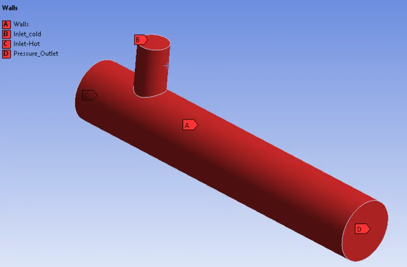
Case 1 (A): - SHORT TEE, HOT INLET – 3M/S, MOMENTUM RATIO 2, K-ESPILON MODEL
In case 1 we are going to simulate short Tee model with hot inlet at 3m/s and inlet temperature of 36℃. The cold inlet velocity is calculated from momentum ration which is given as:
`Momentum Ratio= (Velocity at Cold INLET)/(Velocity at hot INLET)`
As the velocity at hot inlet is 3m/s and momentum ratio is 2, then velocity at cold inlet is 6m/s with temperature at cold inlet is 19℃.
A) Geometry
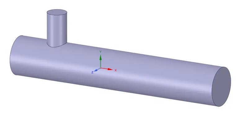
B) Meshing
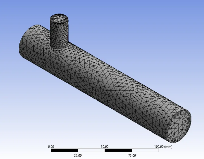
Meshing is done using default feature in ANSYS workbench with 5mm mesh size. The number of element are 21852.
C) Material and Boundary Condition
The fluid used for the simulation is air only. The property of air is given as:
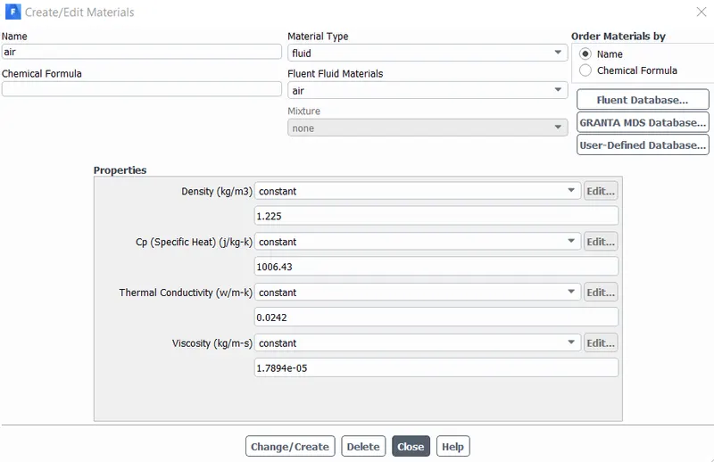
The launch of ANSYS fluent can be done after updating the mesh. We will use double precision option to run simulation x64 bit processor with 8 logical processors.
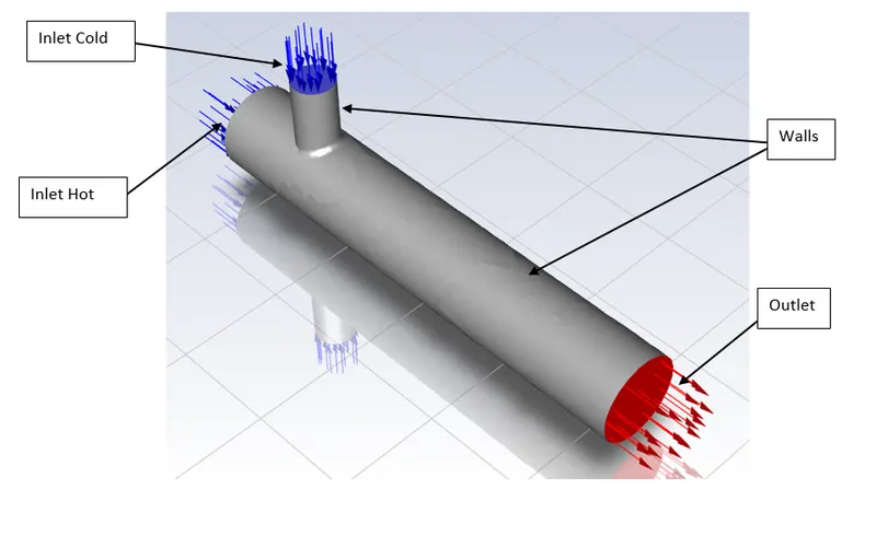
After providing required information for simulation we will create some reports which are important to monitor the solution while iterations. The first report will be of average surface temperature at outlet which will provide use solution of temperature monitoring and other one is standard deviation at outlet which tells us the minimum temperature difference achieve at convergence.
This simulation case 1-A will be performed using K-epsilon turbulence model with standard wall function. After running the simulation, the results are:
D) Post Processing
1) Residual Plot
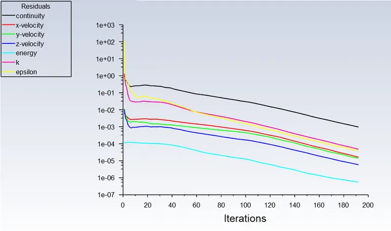
From above image it is confirmed that solution is converged around 200 iteration.
2) Average Temperature at Outlet
3) Standard Deviation at outlet
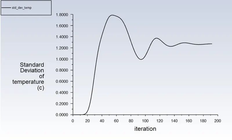
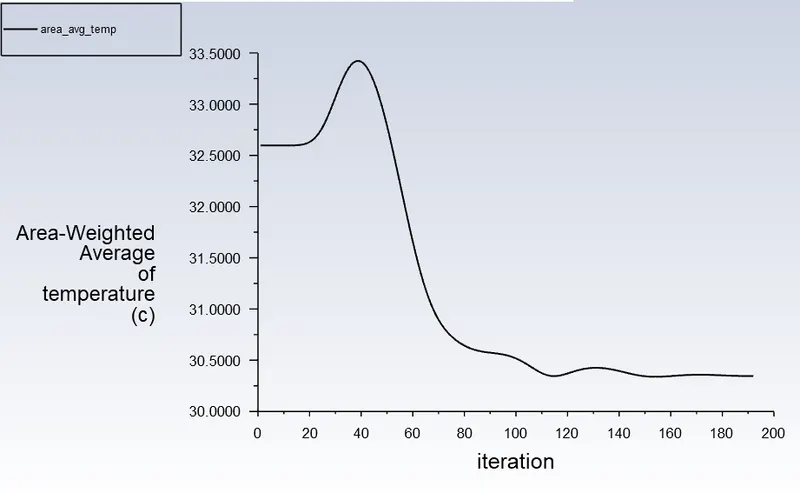
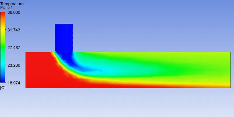
From the plot we can see that the simulation has been converge for 197 iteration and average temperature at outlet is 30.344 ℃ and standard deviation is 1.27.
4) Temperature Plot
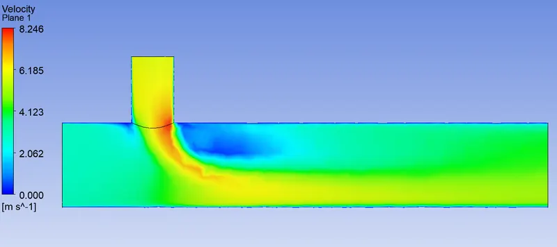
5) Velocity Plot
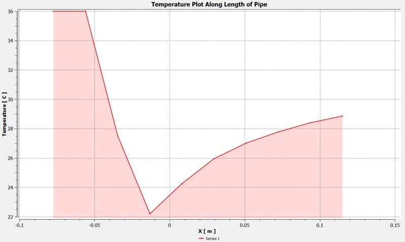
6) Temperature Plot Along length of Pipe
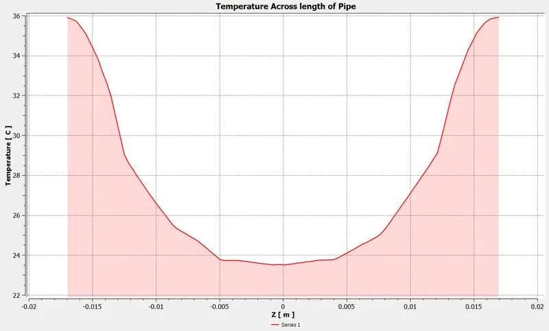
7) Temperature Plot Across Length
8) Velocity Plot Along length
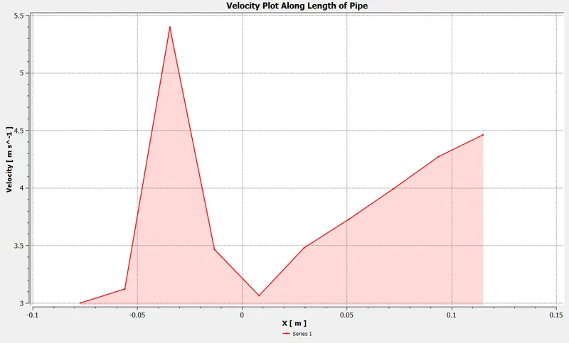
9) Velocity Plot Across length
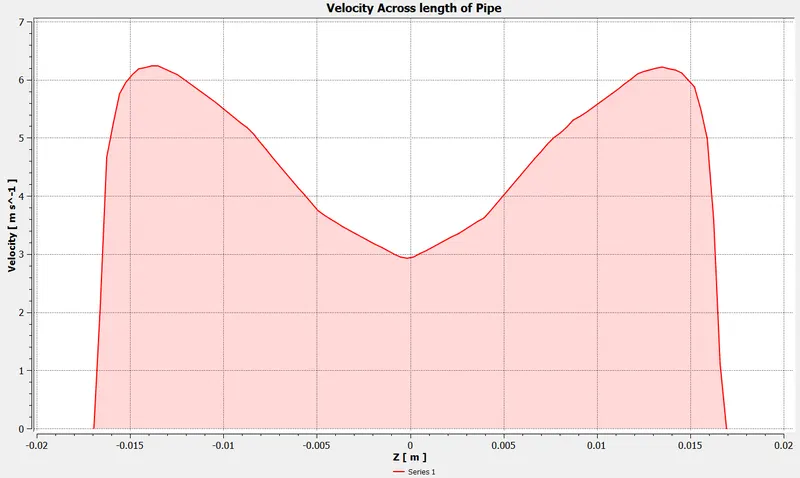
Case 1 (B): - SHORT TEE, HOT INLET – 3M/S, MOMENTUM RATIO 4, K-ESPILON MODEL
A) Post Processing
1) Residual Plot
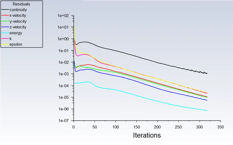
2) Average Temperature Plot
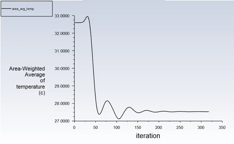
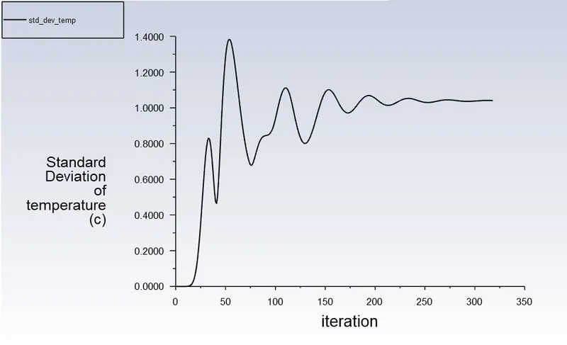
3) Standard Deviation
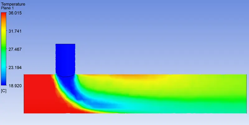
4) Temperature Plot
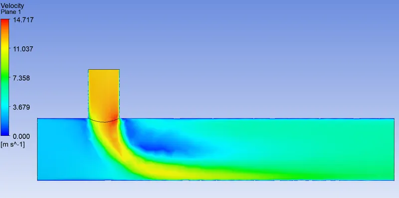
5) Velocity Plot
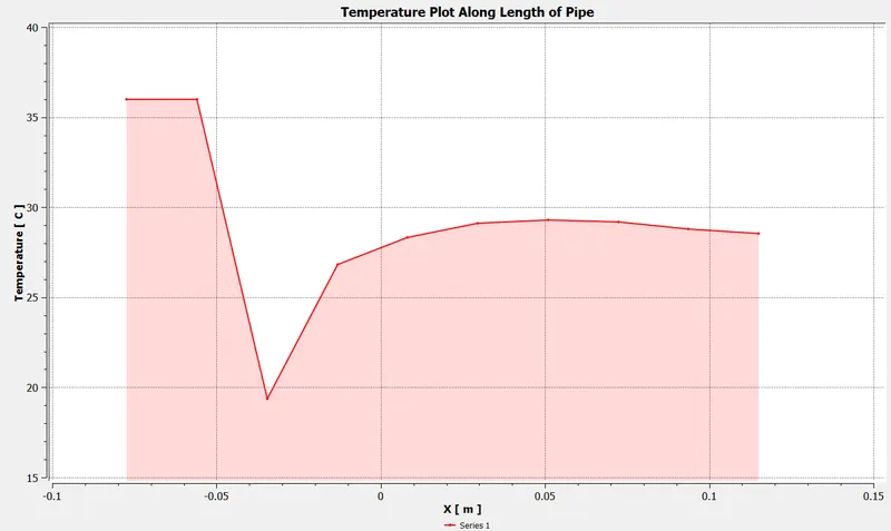
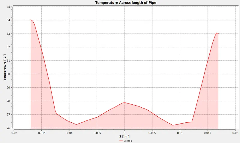
6) Temperature Along length of Pipe
7) Temperature Across length
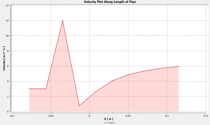
8) Velocity Along length
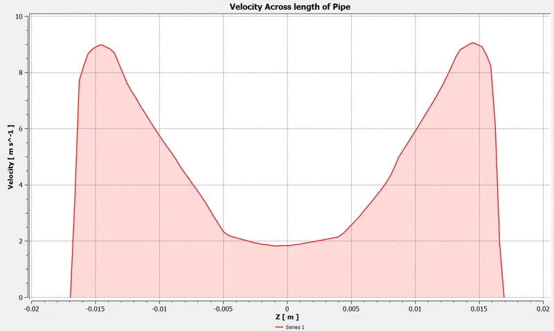
9) Velocity Across length
Case 2 (A): - Long TEE, HOT INLET – 3M/S, MOMENTUM RATIO 2, K-ESPILON MODEL
A) Post Processing
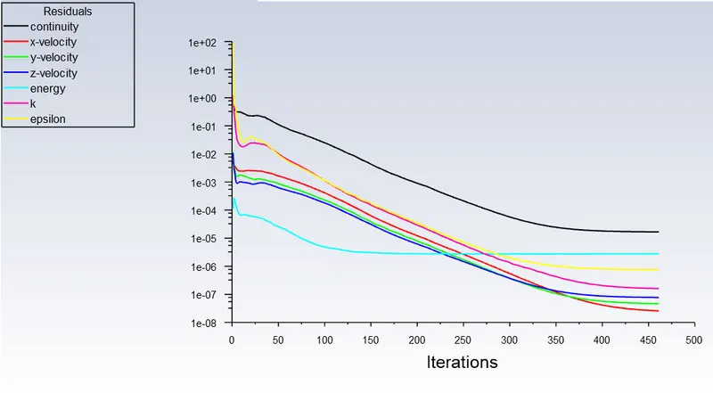
1) Residual
2) Average Temperature
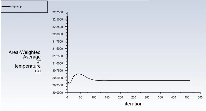
3) Standard Deviation
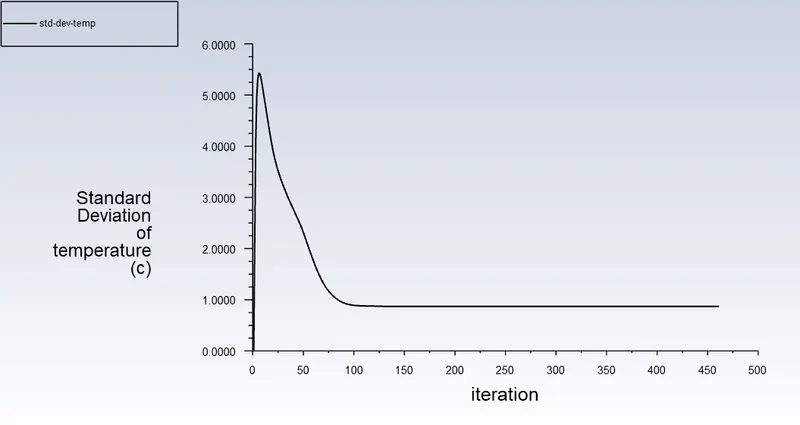
4) Temperature Plot
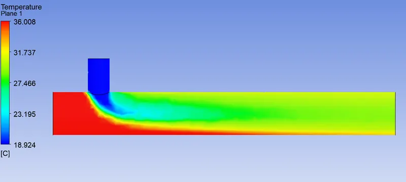
5) Velocity Plot
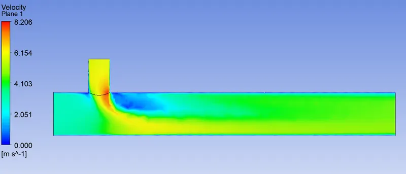
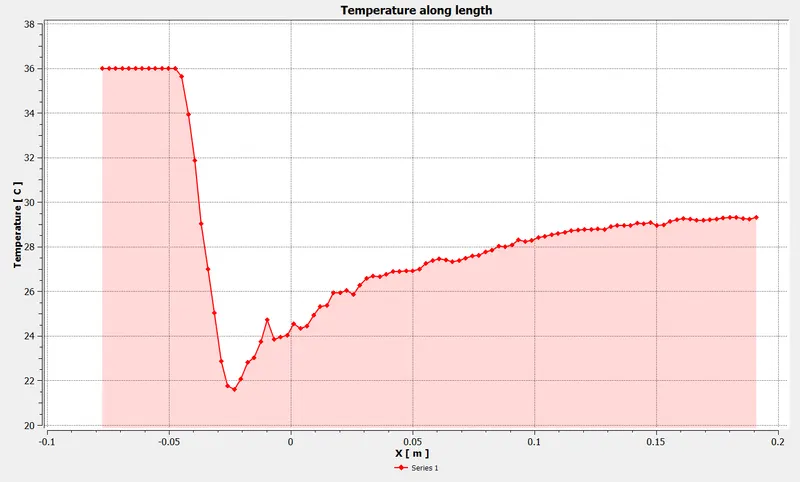
6) Temperature Along length
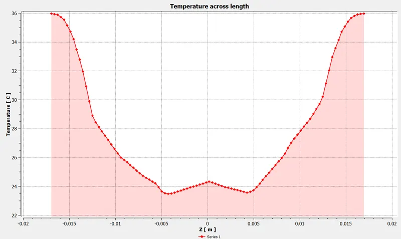
7) Temperature across length
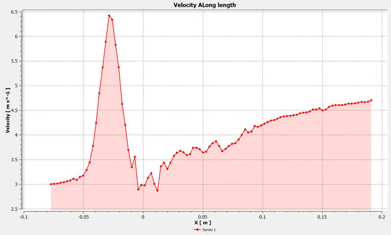
8) Velocity Along length
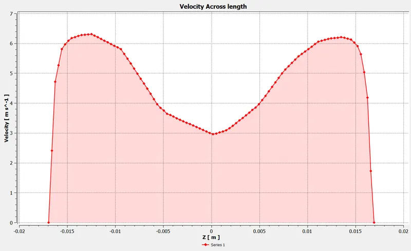
9) Velocity Across length
Conclusion
1) For second case the k-espilon model has been used because of better convergence and lower standard deviation model.
2) The mesh independent test is carried and found that at mesh 1.5 the result are not changing drastically for 2mm mesh outlet temperature is 27.48 for long tee with 4 momentum ration and standard deviation was 0.56. when compared with same case with higher mesh size the results were 30.4 temperature at outlet and 0.86 is standard deviation.
3) The effectiveness of Mixing Tee is not very considerable by changing the length of Tee it was mostly by increasing flow velocity which create better turbulence at outlet.