Week 5.2 - Literature review: ODE Stability
Week 5: - ODE Stability Criteria using Python
Aim: - Evaluation of ODE stability using explicit and implicit Euler methods.
Objective: -
- To study the stability criteria for ODE’s.
- To study explicit approach and its limitation for ODE systems.
- To create a python program for the explicit method of ODE system.
- To study implicit approach and its limitations for ODE system.
- To create a python program for implicit method of ODE system.
- To compare the explicit and implicit approach towards the ODE.
Introduction: -
A differential equation is considering as an ordinary differential equation when the unknown function is depending only upon one independent variable. The exact solutions of differential equations are very hard to evaluate hence the numerical methods has to be introduced to calculate the solution of equation. The stability in the mathematics is the condition in which a small disturbance in the system will not produce too much unsettling an effect on the system. If we consider a system f(x), the function f(x) is said to be stable if any other solution of equation is start out close to it when the x = 0. If the difference between the solution when approaches to zero as x increases, then the solution of equation is called stable. If a solution does not the meet the properties of stabilization it will called as unstable solution.
Stability of solution is essential in the physical problem because the slight deviation from the mathematical model caused by unavoidable errors in system do not have correspondingly effect on the solution, but the prediction of system for future outcome will not be accurate.
Numerical Methods: -
Consider an initial value problem in ODE
`y_t=f(t,y),y(t_0 )=y_0`
where f is the given smooth function. There are numerical methods which provides the information about the solution of equation even if formulas or exact solution cannot be calculated.
- Explicit Method
The forward Euler method is one of the numerical method and is called as explicit in nature or most of the time explicit numerical method. It calculates the state of the system in later time from the state of system at the current time without need to solve algebraic equations. For the forward method, it began by choosing a step size or ∆t. The size of step determines the accuracy of the approximate solution as well as number of computations required. Talking about graphical representations, this method produces a series of line segments, which is approximation solution curve.
Let `t_k,k=0,1,2,…,`be a sequence in time with
`t_(k+1)=t_k+Δt`
Let `y_k`and `Y_k`consider as exact and the approximate solution at time `t = t_k`respectively. To obtain the solution later in time which is `Y_(k+1)` from `(t_k , Y_k)`, we use differential equation. As the slope of solution to equation `y_t = f(t,y)`at point `(t_k , y_k)`is `f(t_k, y_k)`, the explicit Euler method determines the point `(t_(k+1) , Y_(k+1))` by considering that it lies on the line through `(t_k , Y_k)` with the slope `f(t_k, Y_k)`. The formula for slope of the line is given by:
`(Y_(k+1)-Y_k)/(Δt)= f(t_k ,Y_k )`
or
`Y_(k+1)=Y_k+f(t_k ,Y_k ) Δt`
As the time step size decreases then the error between the actual and approximation is reduced. This method of approximate solution is not stable for most of the cases as length of sub interval increases the error also get increased.
- Implicit Method
The implicit method is called as backward Euler’s method which finds the solution by solving an equation having the current state of system and the later one. The equation of implicit approach is given as:
`Y_(k+1)=Y_k+f(t_k ,Y_(k+1) ) Δt`
In above equation it can be seen that `Y_(k+1)`
appears on the both side of equation. The implicit equation is computationally sturdy to solve but are unconditionally stable as compared to the explicit approach. This approach is mostly used for ODE which are stiff in nature.
Example: -
Consider an Initial Value problem which need to be solved using explicit & Implicit approach:
`dy/dx= -1000∙y-e^(-t)`
The analytical solution to the equation is given as:
`y(t)=((e^(-1000t) (1-e^999t )))/999`
- Explicit Code
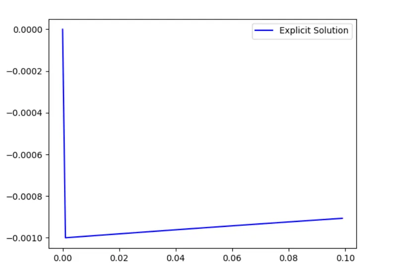
In this code the structure follows with Comments defining title of code and equation solved using explicit method. Then import of ‘numpy’ and ‘matplotlib.pyplot’ is used to operate the program. After that a function is defined in which variable are ‘total_t’ and ‘dt’ are used. Inside the function variables i.e. ‘t’ and ‘y’ are defined using ‘np.arange’ and ‘np.zeros’. The ‘np.arange’ is array generating routine used to create Evenly spaced value. Similarly, ‘np.zeros’ is used to create the value of zeros inside the array for length of ‘t’. Then a loop is created with range operator for find the solution of equation which is stated above. For the solution ‘total_t’ and ‘dt’ is defined for calculation of y with respect to time. After that ‘matplotlib.pyplot’ is used for creating graphical representation of the solution for time as 0.1 and time step size as 1.0e-3. The code is given as follows:
"""
Week 5 - Challenge 5.2
ODE Stability of Initial Value Problem
Code By: - Shubham Chaudhari
Initial Value Equation:
(dy/dx) = -1000 * y - math.exp(-t)
Explicit Approach
"""

import numpy as np
import matplotlib.pyplot as plt

# Defining function for Explicit


def explicit_euler(total_t, dt):
    t = np.arange(0, total_t, dt)   # Creation of Evenly spaced value from 0 to 0.1 with Interval of 1.0e-3
    y = np.zeros(len(t))            # Creation of y solution with all values as Zeros with length of t

# Creating a Loop for solution with range operator
    for i in range(1, len(t)):
        y[i] = y[i-1] + dt*(-1000*y[i-1] - np.exp(-t[i-1]))

    return [t, y]

# Defining Total Time of Solution
total_t = 0.1
# Defining Time step size for solution
dt = 1.0e-3
t, y_explicit = explicit_euler(total_t, dt)
plt.plot(t, y_explicit, color='blue')
plt.legend(['Explicit Solution'])
plt.show()
Result: -
For time = 0.1 and dt = 1.e-3
2. Implicit Code
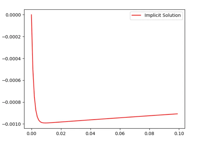
The implicit code follows the same order of explicit code just a change is made in loop which follows below equation:
`y_(i+1)=((y_i-Δt∙e^(-t_(i+1) ) ))/(1+1000∙Δt)`
The code is given as follows:
"""
Week 5 - Challenge 5.2
ODE Stability of Initial Value Problem
Code By: - Shubham Chaudhari
Initial Value Equation:
(dy/dx) = -1000 * y - math.exp(-t)
Implicit Approach
"""

import numpy as np
import matplotlib.pyplot as plt

# Defining function for Implicit


def implicit_euler(total_t, dt):
    t = np.arange(0, total_t, dt)   # Creation of Evenly spaced value from 0 to 0.1 with Interval of 1.0e-3
    y = np.zeros(len(t))            # Creation of y solution with all values as Zeros with length of t

    # Creating a Loop for solution with range operator
    for i in range(1, len(t)):
        y[i] = (y[i-1] - np.exp(-t[i-1])*dt)/(1+1000*dt)

    return [t, y]

# Defining Total Time of Solution
total_t = 0.1
# Defining Time step size for solution
dt = 1.0e-3
t, y_implicit = implicit_euler(total_t, dt)
plt.plot(t, y_implicit, color='red')
plt.legend(['Implicit Solution'])
plt.show()
Result: -
For time = 0.1 and dt = 1.e-3
3. Analytical Method
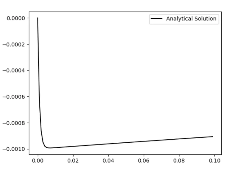
In analytical code the exact solution of equation is used to calculate the y with respect to time t. The following equation is used to calculation of equation.
`y(t)=((e^(-1000t) (1-e^999t )))/999`
The code for analytical calculation is given below:
"""
Week 5 - Challenge 5.2
ODE Stability of Initial Value Problem
Code By: - Shubham Chaudhari
Initial Value Equation:
(dy/dx) = -1000 * y - math.exp(-t)
Analytical Method
"""

import numpy as np
import matplotlib.pyplot as plt

# Defining function for Analytical Method


def analytical_euler(total_t, dt):
    t = np.arange(0, total_t, dt)   # Creation of Evenly spaced value from 0 to 0.1 with Interval of 1.0e-3
    y = np.zeros(len(t))            # Creation of y solution with all values as Zeros with length of t

    # Creating a Loop for solution with range operator
    for i in range(1, len(t)):
        y[i] = np.exp(-1000*t[i])*(1-np.exp(999*t[i]))/999

    return [t, y]

# Defining Total Time of Solution
total_t = 0.1
# Defining Time step size for solution
dt = 1.0e-3
# Plotting of Solution
t, y_analytical = analytical_euler(total_t, dt)
plt.plot(t, y_analytical, color='black')
plt.legend(['Analytical Solution'])
plt.show()
Result: -
For time = 0.1 and dt = 1.e-3
4. Comaprison of All Method
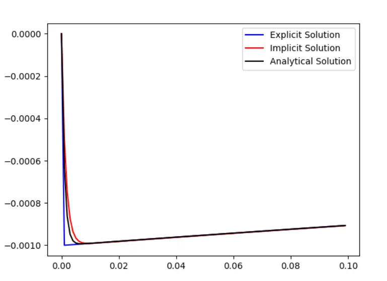
In this code we will compare the explicit, implicit and analytical method for different time step size so that we can see that for larger time interval the implicit method is more stable as compared to explicit one and which is validated by the analytical solution of equation. The code for the 0.1-time step of all methods are given as follows:
"""
Week 5 - Challenge 5.2
ODE Stability of Initial Value Problem
Code By: - Shubham Chaudhari
Initial Value Equation:
(dy/dx) = -1000 * y - math.exp(-t)
All method (Explicit, Implicit & Analytical Methods)
"""

import numpy as np
import matplotlib.pyplot as plt

# Defining function for Explicit


def explicit_euler(total_t, dt):
    t = np.arange(0, total_t, dt)   # Creation of Evenly spaced value from 0 to 0.1 with Interval of 1.0e-3
    y = np.zeros(len(t))            # Creation of y solution with all values as Zeros with length of t

    # Creating a Loop for solution with range operator
    for i in range(1, len(t)):
        y[i] = y[i-1] + dt*(-1000*y[i-1] - np.exp(-t[i-1]))

    return [t, y]


# Defining function for Implicit Method


def implicit_euler(total_t, dt):
    t = np.arange(0, total_t, dt)   # Creation of Evenly spaced value from 0 to 0.1 with Interval of 1.0e-3
    y = np.zeros(len(t))            # Creation of y solution with all values as Zeros with length of t

    # Creating a Loop for solution with range operator
    for i in range(1, len(t)):
        y[i] = (y[i-1] - np.exp(-t[i-1])*dt)/(1+1000*dt)

    return [t, y]


# Defining function for Analytical Method


def analytical_euler(total_t, dt):
    t = np.arange(0, total_t, dt)   # Creation of Evenly spaced value from 0 to 0.1 with Interval of 1.0e-3
    y = np.zeros(len(t))            # Creation of y solution with all values as Zeros with length of t

    # Creating a Loop for solution with range operator
    for i in range(1, len(t)):
        y[i] = np.exp(-1000*t[i])*(1-np.exp(999*t[i]))/999

    return [t, y]

# Defining Total Time of Solution
total_t = 0.1
# Defining Time step size for solution
dt = 1.0e-3
# Plotting of Solution
t, y_explicit = explicit_euler(total_t, dt)
plt.plot(t, y_explicit, color='blue')
t, y_implicit = implicit_euler(total_t, dt)
plt.plot(t, y_implicit, color='red')
t, y_analytical = analytical_euler(total_t, dt)
plt.plot(t, y_analytical, color='black')
plt.legend(['Explicit Solution','Implicit Solution','Analytical Solution'])
plt.show()
Result: -
For time = 0.1 and dt = 1.e-3
For Time = 0.1 and dt = 1.5e-3
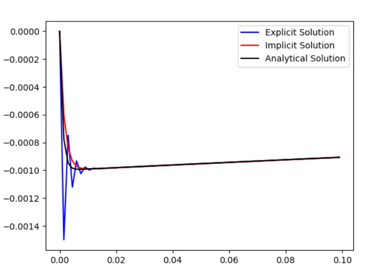
Observation and Conclusion:
1) From the explicit method for 1.0e-3 time step we can see that the curve is very stiff from start to end whereas in case of explicit method it is more smooth for same time step. When compared with analytical method the implicit curve is matched in every respect whereas there is more error when compared to explicit method.
2) For the increase time step size we can see the explicit method has gone unstable whereas implict method still follow the analytical solution curve. This shows that for bigger time step size the implicit method more stable as compared with explicit.
Question 1: - When Does ODE become Unstable
Answer: - The ODE become unstable for the explicit scheme when the time step size is increase from 1.0e-3 to 1.5e-3. The explicit method solution for ODE can become unstable if the time for solution is reduced.
Question 2: - How does stability affect engineering simulations?
Answer: - Consideration of engineering simulation, stable solution will bring equilibrium for the problem and the further state of solution can be predicted accurately. If the solution is oscillating for the initial stage and then oscillation are dying down for rest of the case those solution can be accepted depending upon the criteria of solutions. In most of the engineering problem, the differential equation are used to find state of solution after certain time interval. Using numerical integration technique lowers the error produced in the simulation which has to be key aspect of stability criteria.
Question 3: - Can stability condition be derived for all types of problems?
Answer: - Stability conditions can be used for problems where approximations are made. Most of linear ODE can be solved by stability conditions. For non-linear ODE jacobian methods are used.