Performing a System level Simulation on a CVT BAJA ATV model

AIM : To carry out a system-level simulation of the available All-Terrain Vehicle (ATV) model and to prepare a detailed technical report on the same.

THEORY :

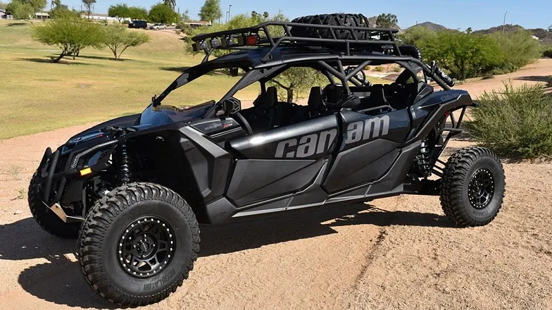
An all-terrain vehicle (ATV), also known as a quad (cycle), three-wheeler, four-track, four-wheeler, or quadricycle, as defined by the American National Standards Institute (ANSI) is a vehicle that travels on low-pressure tires, with a seat that is straddled by the operator, along with handlebars for steering control. As the name implies, it is designed to handle a wider variety of terrain than most other vehicles.

By the current ANSI definition, ATVs are intended for use by a single operator, although some companies have developed ATVs intended for use by the operator and one passenger. These ATVs are referred to as tandem ATVs.

The rider sits on and operates these vehicles like a motorcycle, but the extra wheels give more stability at slower speeds. Although most are equipped with three or four wheels, six-wheel models exist for specialized applications.

SOLUTION :

This model uses a CVT (Continuously Variable Transmission) subsystem.

What is a CVT ?

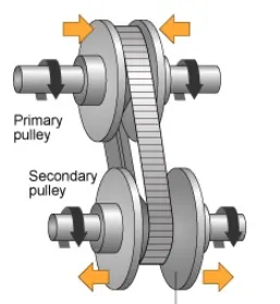
A 'Continuously Variable Transmission' is an automatic transmission that can change seamlessly through a continuous range of gear ratios. This contrasts with other transmissions that provide a limited number of gear ratios in fixed steps. The flexibility of a CVT with suitable control may allow the engine to operate at a constant RPM while the vehicle moves at varying speeds.

CVTs are used in automobiles, tractors, motor scooters, snowmobiles and earthmoving equipment.

The most common type of CVT uses two pulleys connected by a belt or chain, however several other designs have also been used at times.

CVT Subsystem :

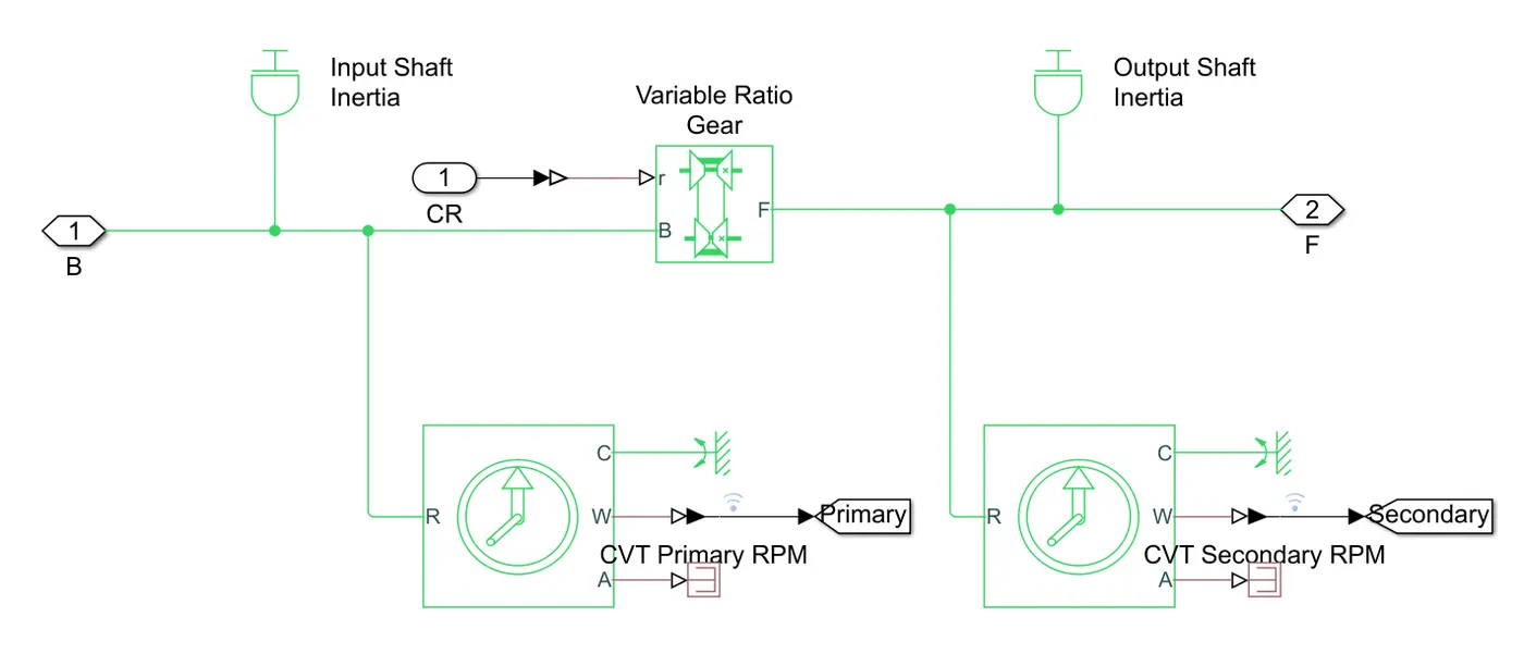
• The CVT subsystem uses a Variable Gear Ratio block.
• Inside the CVT subsystem, 2 Inertia blocks are connected to ensure proper inertial motion.
• Two Ideal Rotational Motion Sensors are connected, one on either side of the Variable Gear Ratio. The angular velocity outputs of these are then transferred to the main model with the help of GoTo blocks.

Vehicle Subsytem :

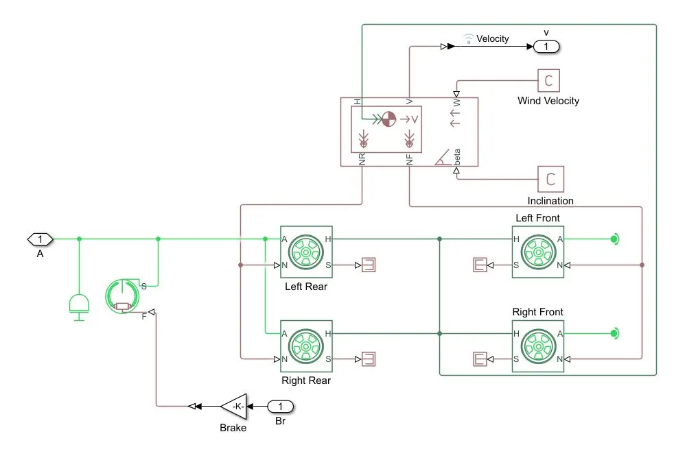
• The Vehicle Body block represents a two-axle vehicle body in longitudinal motion. The block accounts for body mass, aerodynamic drag, road incline, and weight distribution between axles due to acceleration and road profile.
  Mass - 250kg
  Distance between CG to Front Axle - 1m
  Distance between CG to Rear Axle - 0.35m
  Height of CG above ground - 0.7m
• Each of the axles consist of two wheels.
  Rolling Radius - 0.2794m
  Rolling Resistance - 0.015
• The rear wheels share the same rotational motion so their corresponding rotational ports are connected. Since, the front wheels are freely rotating, their rotational ports are connected to Rotational Free Ends. These can be mutually connected too.
• Since, all the wheels share the same translational motion, the corresponding ports of all the wheels are connected to each other.
• The driver shaft is given proper rotational input through an Inertia (Inertia = 1e-1 kg*m^2) block along with the brake input through a Double Shoe Brake.
  Drum Radius - 150mm
  Shoe Span Angle - 120°
• The Velocity of the Vehicle Body is taken out as an output in order to get visualised in the main body.
  
  

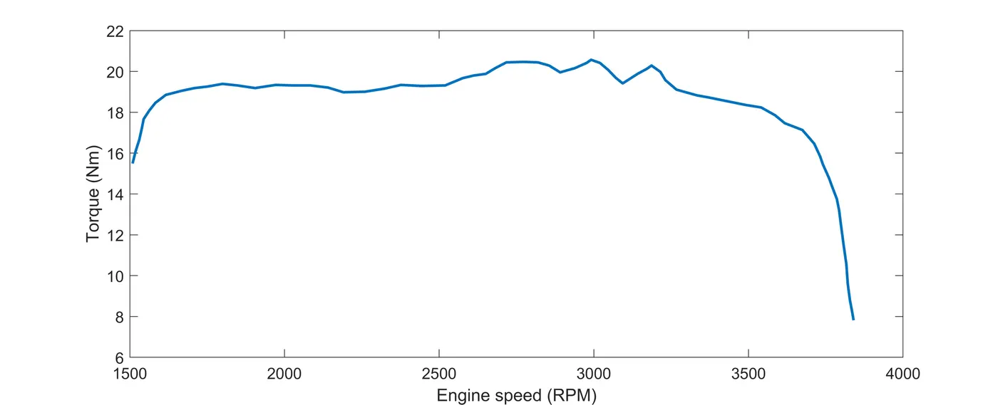
Plot of 'Engine Torque v/s Speed' :

Now, depending upon the different types of inputs, five different model simulations are carried out.

Model 1. (A) : cvtModel

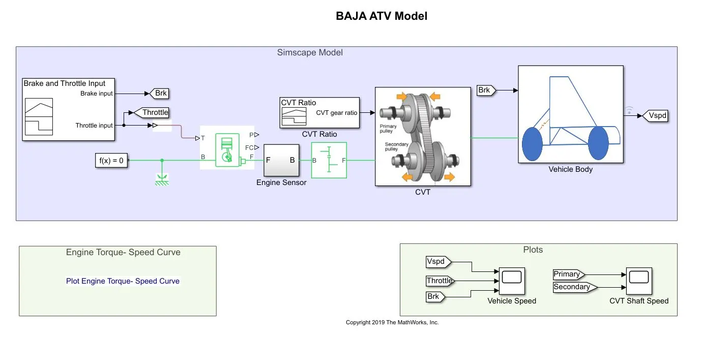
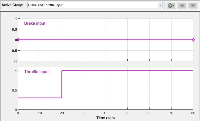
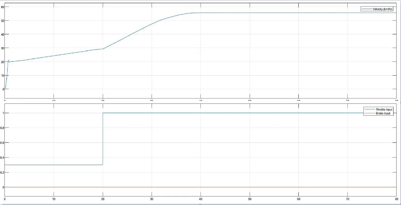
• In this model, the Brake and Throttle inputs are given with the help of a Signal Builder block. Here, the brake input value is kept 0 throughout and just the throttle input is given a rise, at t=20 sec, to study the variation of the vehicle speed.
  
  
  
  
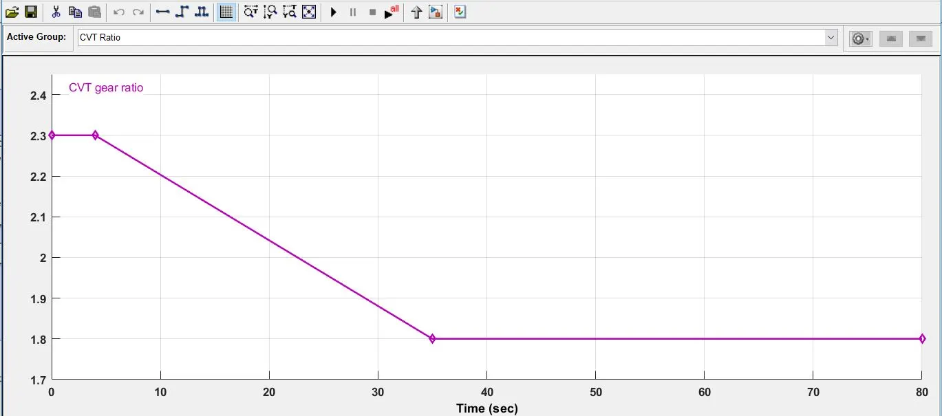
• The input CVT Ratio is also given with the help of another Signal Builder block. Its value remains constant at 2.3 for first 4 sec, then is reduced linearly to 1.8 at t=35 sec.
  
  
  
  

Result/Output :

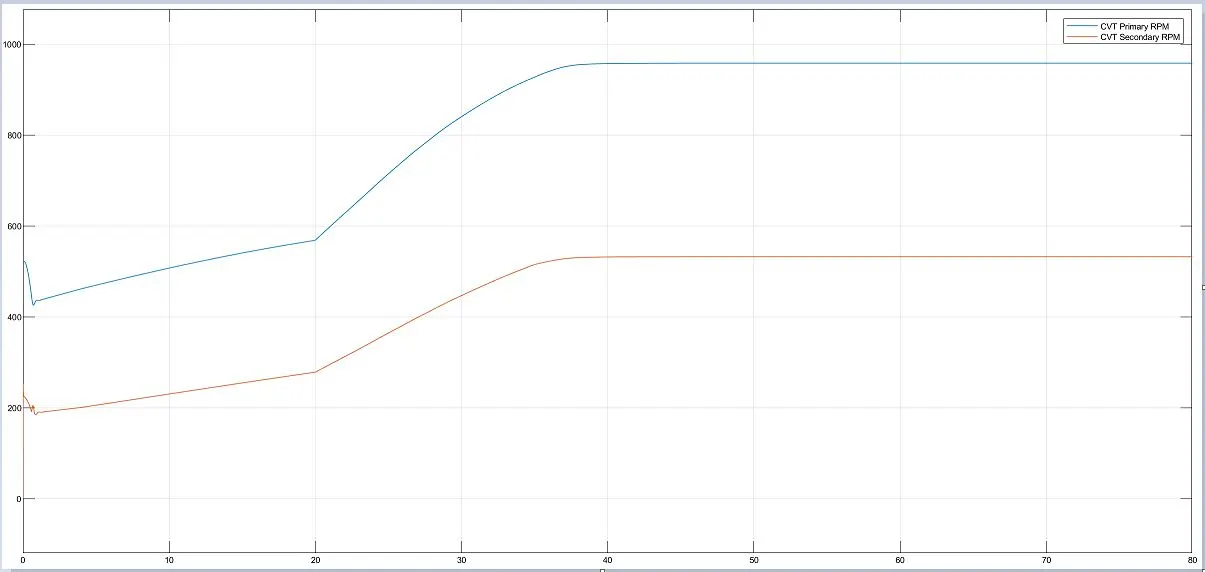
• These are the angular velocities before and after the Variable Gear Ratio coming into play in the CVT subsystem.
  
  
  

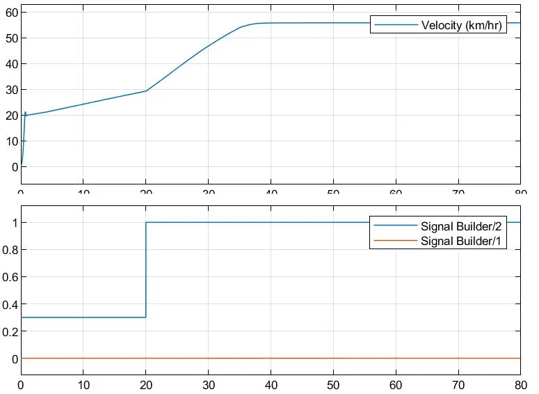
• The 2 signal builder plots are nothing but the Brake and Throttle inputs given to the model.
• The Vehicle speed varies as shown in the plot. Due to the initial throttle of 0.3 units, the vehicle shows a sudden rise in the velocity at the start. For the next 20 sec of constant throttle, the vehicle speed gradually increases up until the point where the throttle is given a complete push. The vehicle accelerates at a higher rate till it reaches the top speed.
  
  

Model 1. (B) : cvtModel_Dashboard

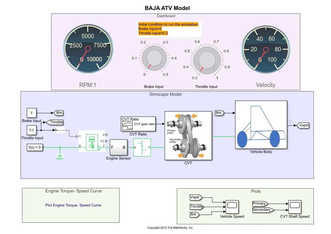
• The only difference between this and the previous model simulation is - instead of giving a signal builder inputs of Brake and Throttle, these are provided by connecting Knobs.
• This enables us to run the model as per Real time simulation, wherein the input can be varied while the simulation is running.
• Accordingly, the stop time is set to infinite.

Result/Output :

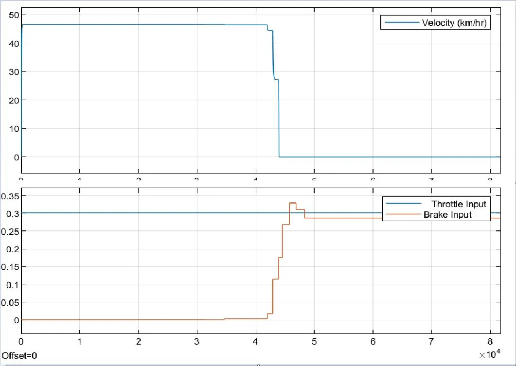
• While the simulation is being run, the Brake was applied at around t=4 sec, while keeping the throttle input constant, the velocity of the vehicle quickly falls down to 0 i.e it comes to rest.
  
  
  

The next three models are based upon taking the input values for the CVT subsystem from a Lookup Table which is itself created in one of the models.

Model 2. (A) : cvtModel_data

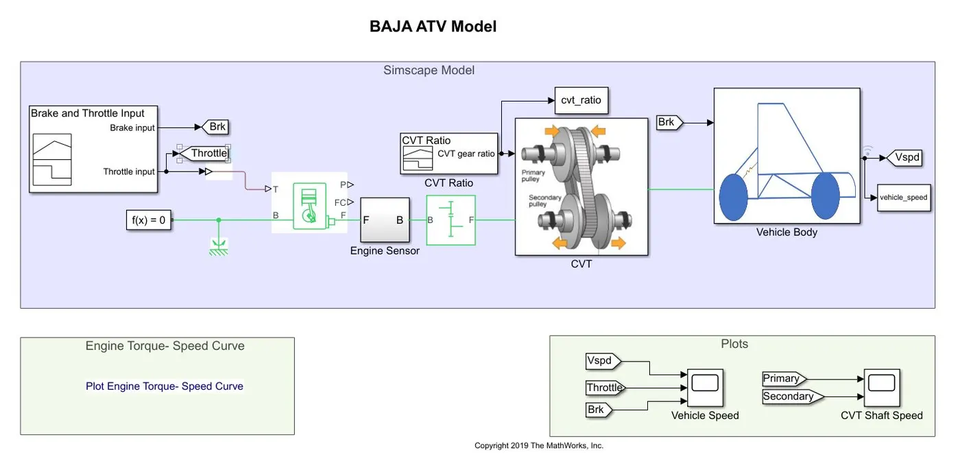
• This is the same as model 1. (A) discussed above.
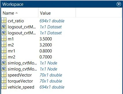
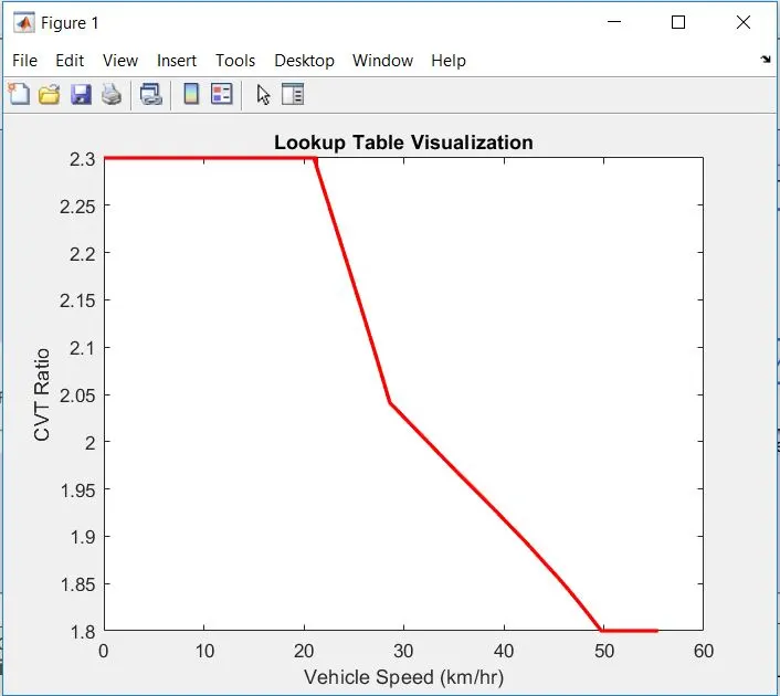
• Here, the Lookup Table is created by taking the values from the CVT Ratio block and the final velocities of the vehicle corresponding to the CVT Ratio values. The To Workspace blocks are used for this purpose.
• By running the model, the values of the Lookup table are stored in the Base Workspace.
  
  

Lookup table visualisation -

Model 2. (B) : cvtModel_mapped

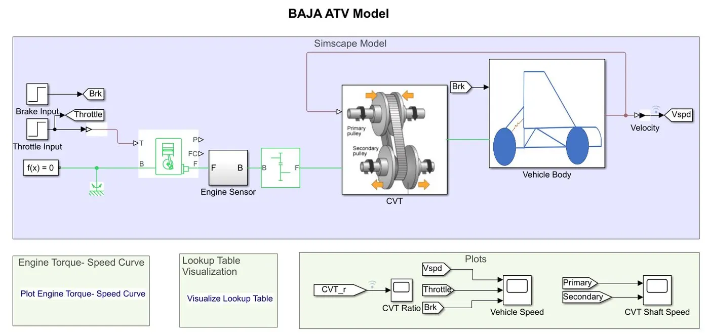
• This model takes input for the CVT subsystem from the Lookup Table created in the previous model, instead of the Signal Builder block used earlier.
  
  
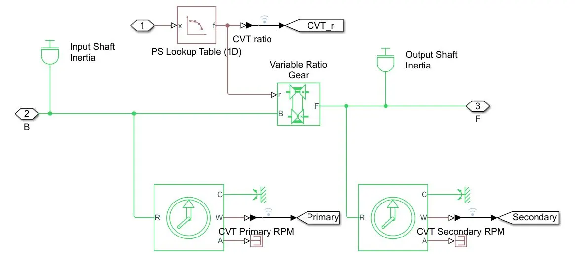
• GoTo and From blocks are used in order to visualize the values of CVT Ratio in the output.
  
  

Result/Output :

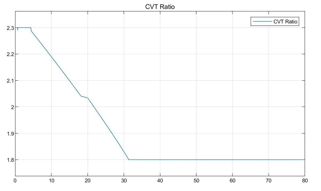
• Since, the values of the Lookup table are already taken from the initial models, the final result velocity plot is inturn, similar to the earlier one.
  
  
  
  
  

Model 2. (B) : cvtModel_dashboard_mapped

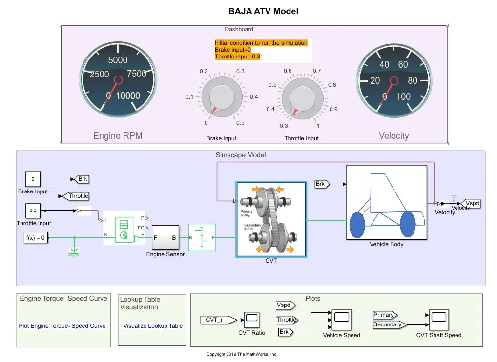
• This model, as the name suggests, is similar to the model 1. (B), wherein the Brake and the Throttle inputs are given from Knobs. (Real time simulation)
• Also, the model uses the Lookup table for the CVT Ratio values.

Result/Output :

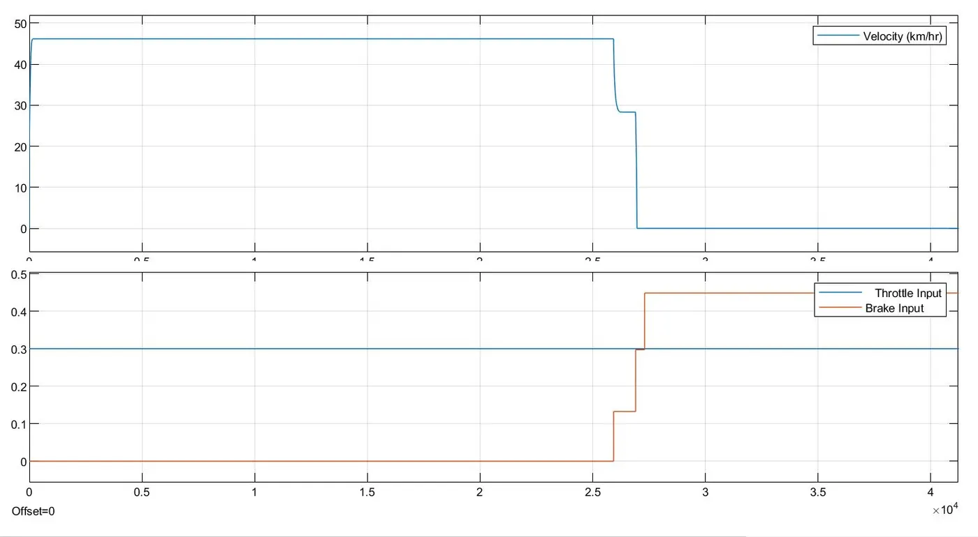
• The simulation is run while keeping the Throttle input constant. Brake is applied at t=2.5 sec, accordingly, the vehicle comes to rest quickly.

CONCLUSION :

A system level simulation was performed on the ATV model and the models along with the simulation results were studied succesfully.