Crash Simulations of a Ball & Plate using different material cards in Radioss

AIM : To perform simulations on the given models as per the required properties and to compare all the 7 cases.

OBJECTIVES :

1. To run the provided FAILURE_JOHNSON model for simulation as it is.
2. To remove the plastic strain failure value and add a failure Johnson card with the recommended card flag values.
   Ifail_sh=1; Dadv=1; Ixfem=1
3. To delete the Johnson failure card and run the model as Law2_epsmax_nofail.
4. To delete the eps_p_max value and run the model with name Law2.
5. To convert this material model to Law1 elastic with same density, E,nu values and run the simulation.
6. To change the shell properties to recommended values in the provided LAW27 file and run the mode with name LAW27.
7. To convert the card to Law36 elastoplastic material as per the recommended properties.

Based on the results and outputs of each of the simulation cases, the following tasks are to be performed.

(a) To compare the 7 cases on the basis of - Total number of cycles, Energy Error, Mass error and Simulation time.
(b) To notice the animation of all 5 simulations and describe the animations in brief on the basis of whether the elements are being deleted or cracked.
(c) To plot energies and notice any difference.
(d) Based on all the results, state which case would represent the on-field scenario.
(e) To prepare a report and list down case by case result and conclude as to why the failure happened.

SETUP & PROCEDURE :

Case I : To run the provided FAILURE_JOHNSON model for simulation as it is.

• The provided Started file (.rad) is imported in Hypermesh.
• For this base simulation, the properties i.e. both the element formulation and material properties are left with their default values.
  
  
  
  
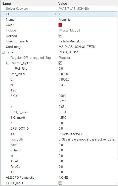
• The default material card is the Johnson-Cook elasto-plastic material i.e. M2_PLAS_JOHNS_ZERIL.
  Here, all the values are in g-mm-ms system which can be seen in the BEGIN_CARD.
  Accordingly,
  density (rho) = 0.0028 g/mm^3 = 2800 kg/m^3
  elastic modulus (E) = 71000 MPa = 71 GPa
  Poisson's ratio (nu) = 0.33
  Yield stress (SIGY) = 290 MPa
  Max. Plastic Strain (EPS_p_max) = 0.151 MPa
  Plastic hardening parameter (b) = 562.3
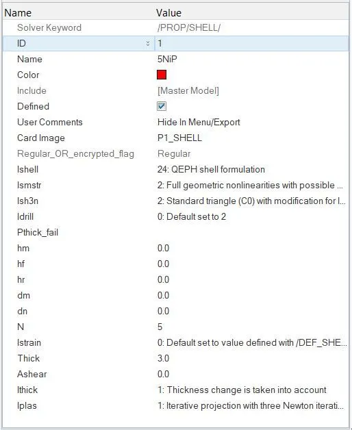
  Plastic hardening exponent (n) = 0.63
  
  
• In the property card, P1-SHELL card image is chosen since the plate is modelled with quad shell elements.
• The element formulation is done as per the optimal choices such as Ishell = 24 which is for QEPH integration method.
  Since, the simulation involves high deformation, the Ismstr = 2 which corresponds to large strain formulation by considering the instantaneous values.
  The number of integration points N is kept as 5.
  To account for the thickness change over the elements, Ithick = 1 is chosen.
  Also, to consider the stiffness change over the thickness due to the plastic strain involved, Iplas = 1 is chosen.
• The failure property card used in this simulation is shown below -
  
  
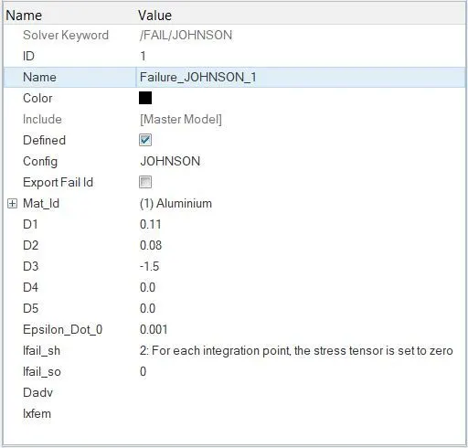
  Here, the values of D1, D2, D3 correspond to the behaviour of the stress-strain curve beyond the Yield limit. The curvature of this curve is governed by the value of Epsilon_Dot_0
  
  Note :The purpose of providing is, essentially, letting the software consider the type of element failure as well. This is basically due to the fact that the elements failing under compression can generally absorb a lot more energy than those failing under tension.
  
  
• Since, the Ixfem flag is not chosen here, it means the failed elements will get completely deleted rather than Radioss showing a crack generated at such places.
  
  
• Now, the Trun, Tstart and Tfreq are provided so as to generate the animation files over the simulation run properly.
  This is done using the ENG_RUN and ENG_ANIM_DT cards respectively.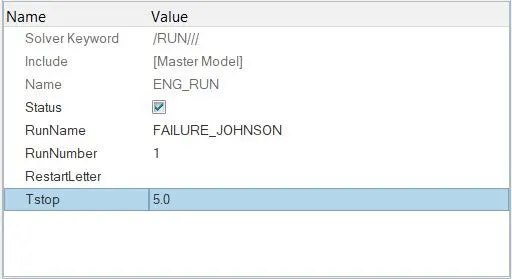
  
  
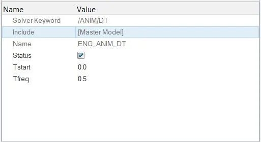
  Accordingly, 10 animation steps will be created.
  
  

Results :

• By running the .H3D animation output file in HyperView, the animation can be visualized.
  
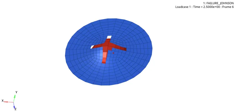
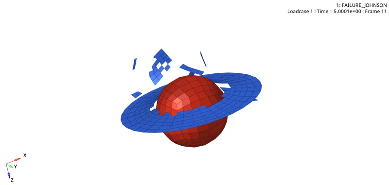
  As we can see, the plate failure is shown by HyperView by simply deleting the failed elements. This is due to the fact that Ixfem flag is not considered here.
  
  
• The enrgy error at the end of simulation is found to be around +0.8% which is quite acceptable considering there is not hourglass enerrgy involved here.
  Also, the mass error remained 0.00 throughout.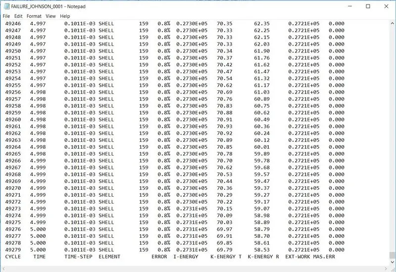
  
  
  
• The failure initially begins at the center and gradually propagates in mutually perpendicular directions.
  This can be effectively visualized by plotting the Von-Mises stresses developed over the plate during the simulation run.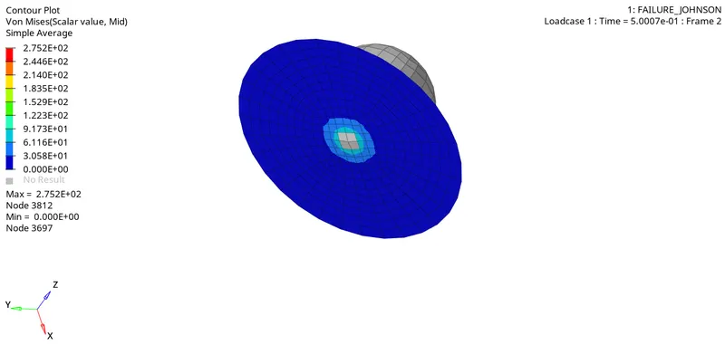
  
  
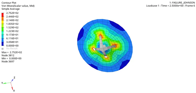
  The maximum plastic strain during the simulation was found to be around 275.2 MPa.
  
  
• Similarly, different output plots can be created in HyperGraph 2D window.
  
  
  
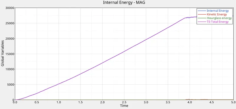
  As the QEPH mode of integration was chosen (Ishell = 24), there is no hourglass energy creation.
  The Internal energy of the plate goes on increasing nearly upto 4 sec after which it shows a fairly constant behaviour.
  The plot of internal energy of plate almost overlaps the total energy plot of the ball.
  
  Plot of Rigid wall forces shows a fluctuating nature during the impact as shown below.
  After that, its magnitude decreases sharply, rightly so, as the most of the ball part has went right past the plate after the impact.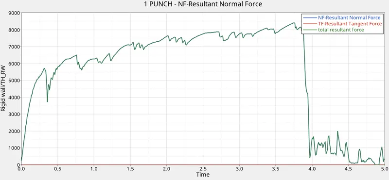
  
  The resultant force graph almost overlaps the graph of normal force. This is due to the fact that there is very less surface area of the ball in contact with the plate during the simulation which in turn results in a very small magnitude of frictional force.
  
  
• Number of cycles = 49279
  Simulation time = 55.78 s which can be seen at the bottom of the engine output file.

Case II : To remove the plastic strain failure value and add a failure Johnson card with the recommended card flag values.
Ifail_sh=1; Dadv=1; Ixfem=1

• Here, the failure card is modified as required.
  Rest all the parameters are left with their initial values.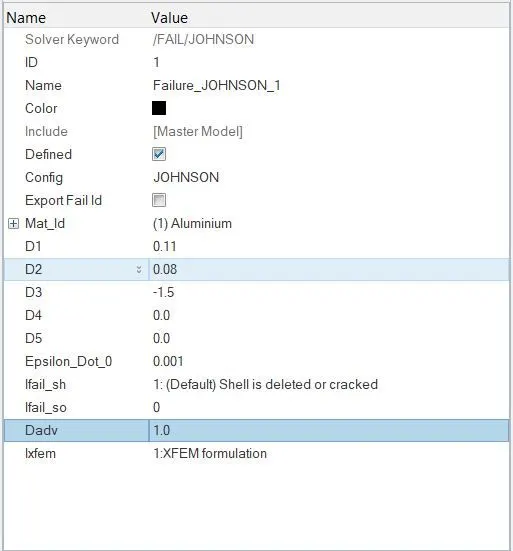
  
  
  
  
• Here, since, the Ixfem flag is enabled, Radioss will show the element failure by generating a crack and not by totally deleting the failed elements.
• The file is exported as per the required name 'law2_epsmax_crack' and saved in .rad format.
• This file is now ran for simulation in Radioss by creating a separate local directory for the ouput files.
  
  

Results :

• The H3D file is loaded in HyperView to visualize the animation.
  
  
  
  
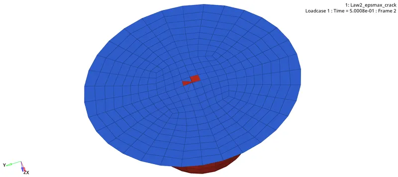
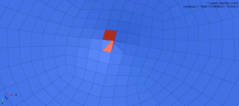
• As we can see, there is crack initiation at the start of the failure instead of directly deletion of the failed elements.
  
  
• Von mises contour is generated in HyperView window.
  
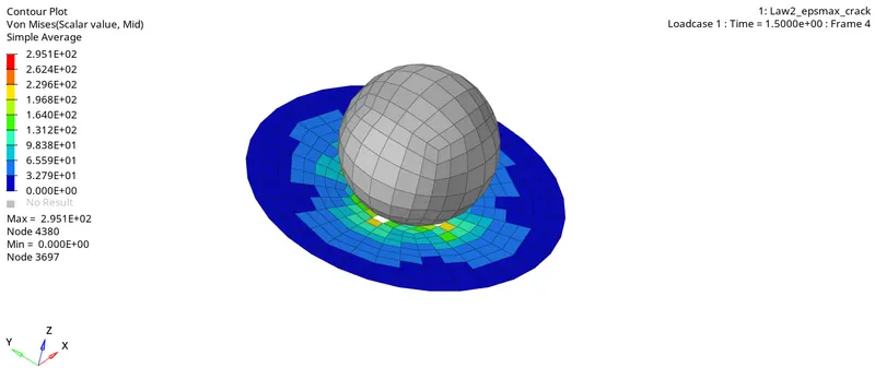
  Here, max. stress = 295 Mpa.
  
  
• The plots for energies and rigid wall forces are shown below.
  
  
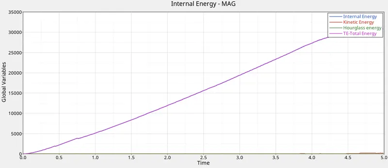
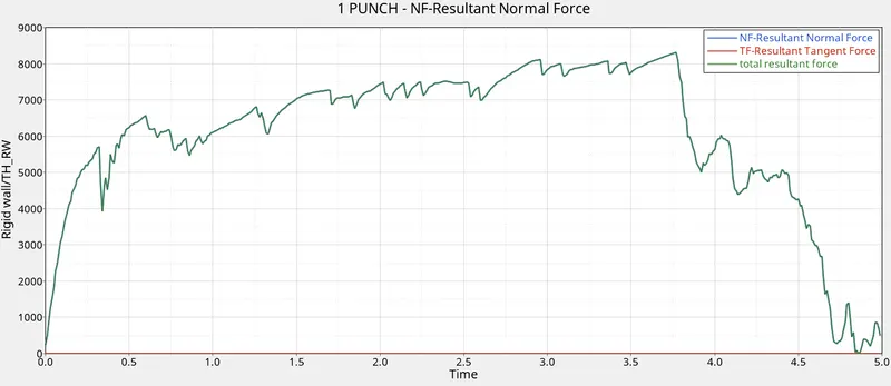
  These plots are pretty much the same as we got in the earlier case.
  
  
• The energy error in this case reached upto 4.0% at the end of simulation. The mass error is 0.00 is this case as well.
  
  
  
  
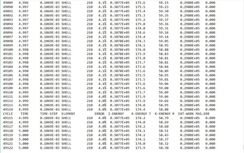
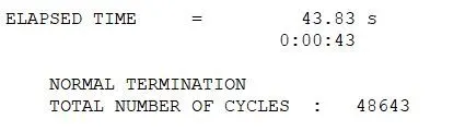
• Here, the number of cycles = 49122 and simulation time elapsed was about 66.16 s

Case III : To delete the Johnson failure card and run the model as Law2_epsmax_nofail

• In this case, the failure card has to be deleted.
  All the other parameters are left with the values in the first case.
  Since, there is no failure card, Radioss will not consider the mode of failure i.e. tension or compression as discussed earlier.
  
  

Results :

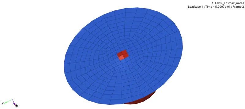
• In this simulation as well, the failure initiation happens directly with the deletion of element as shown below.
  
  
  
  
• The von mises stress contour shows the variation of stress in the plate during the simulation.
  
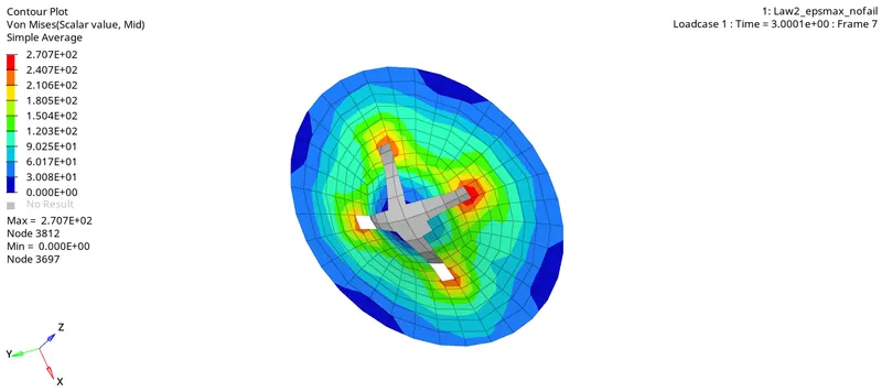
  The maximum stress is 270.7 MPa.
  
  
• Energy plots and rigid wall force plots are shown below.
  The plots show similar nature as in the previous cases.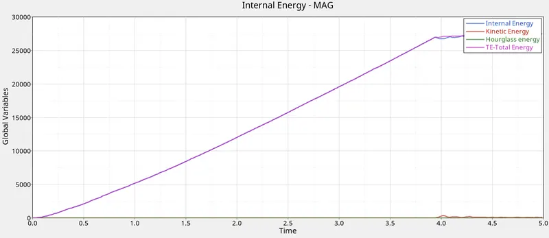
  
  
  
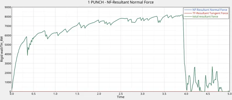
• The energy error in this case, at the end, is found to be much lesser than the previous case 0.8%.
  The mass error is still the same i.e 0.00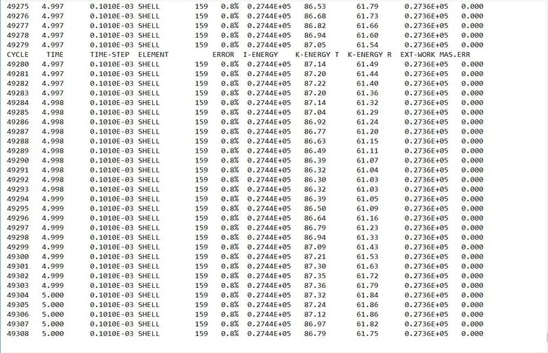
  
  
  
  
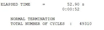
• The number of cycles and simulation time is shown below
  

Case IV : To delete the eps_p_max value and run the model with name Law2

• In this case, we have to remove the maximum plastic strain value from the material card.
  Also, to top that, the failure card is not available in this case too, just like in the previous case.
• Since, the plastic strain failure criteria is absent here, the solver assumes a default value as eps_p_max = 10^30.
• The file is exported in .rad format with the name Law2 and then ran for the simulation.
  
  

Results :

• Here, since we did not specify the failure plastic strain value, Radioss assumed a very high default value for it i.e. 10^30.
  This means, that the material will absorb tremendous amount of energy before its elements even start failing.
  Accordingly, in this case, no element failure is abserved.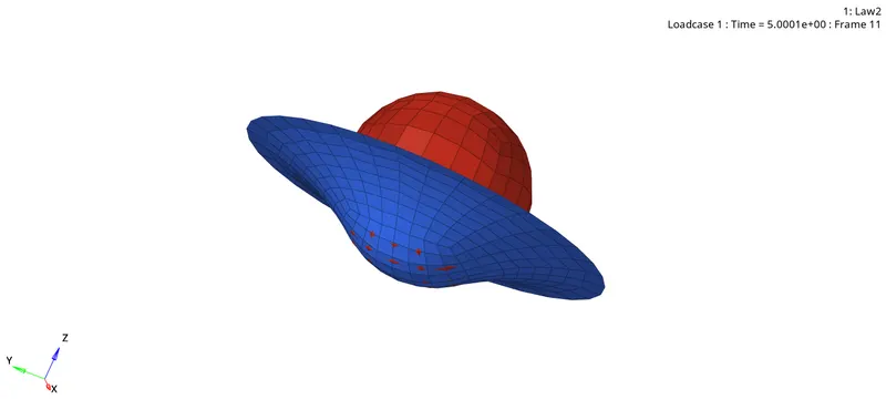
  
  Note : A point here to be noted is that the absence of failure in this simulation case does NOT mean that the material is behaving as an elastic material.
  The deformation happening in this case is still plastic in nature.
  
  
• The plots for energies and the rigid wall forces are generated by using the T01 file in HyperGraph 2D window.
  
  
  
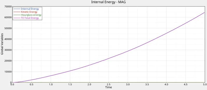
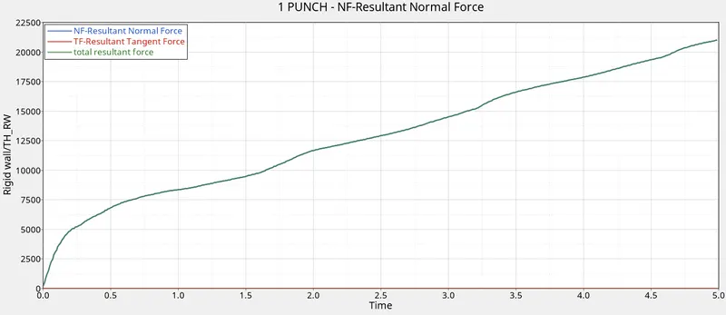
  The plots in this case show a much different behaviour than that in the earlier cases.
  The Internal energy goes on increasing till the end of the simulation, rightly so, as the material has not failed yet and still can absorb energy.
  The rigid wall forces, in this case, do not show fluctuating nature as there is no failure and deletion of elements in this case.
  
  
• The von mises stress variation is much organized in this case with the core section being the most stressed.
  
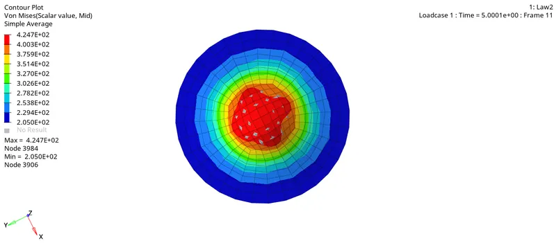
  This must be because there is no crack propagation which would lead to unorganized stress behaviour.
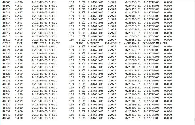
  The maximum stress being about 424.7 MPa (much higher than the previous cases).
• The energy error and mass error values at the end of simulation are 3.0% and 0.00 respectively.
  
  
  
  

Case V : To convert this material model to Law1 elastic with same density, E,nu values and run the simulation

• The new material card with M1_ELAST card image is shown below.
  The material properties are kept the same.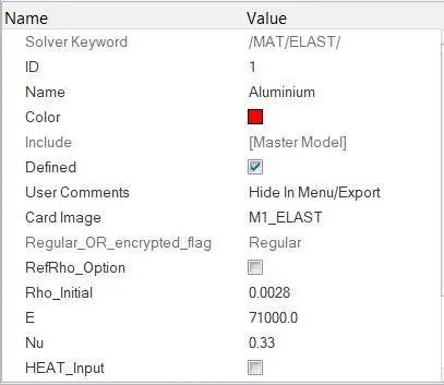
  
  
  
  
• The model is exported with the name Law1 and then ran for simulation.

Results :

• Since, the material card used here is Elastic, it is obvious that the material behaves linearly throughout and there is no plastic deformation of elements, let alone failure.
  
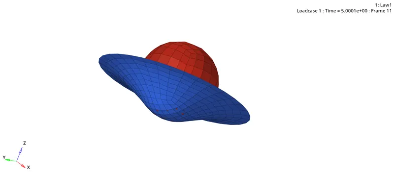
• The Von Mises stress contour in this case shows much similar variation as in the previous case.
  
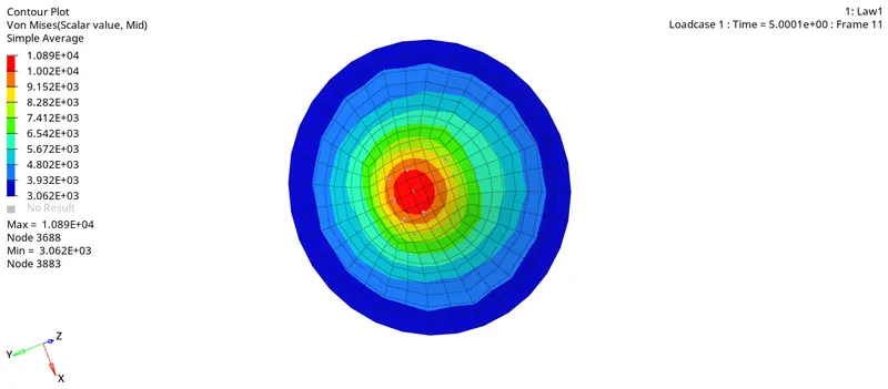
  However, the stress values are much larger in this case.
  This shouldn't be much of a surprise, since, there is no plastic deformation, and so there is no plastic energy dissipation.
  In turn, the material itself has to resist the occuring deformation in the elastic zone only.
  The maximum stress developed here is 1089 MPa.
  
  
• Plots for energies and rigid wall forces -
  
  
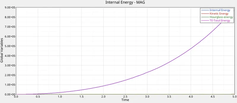
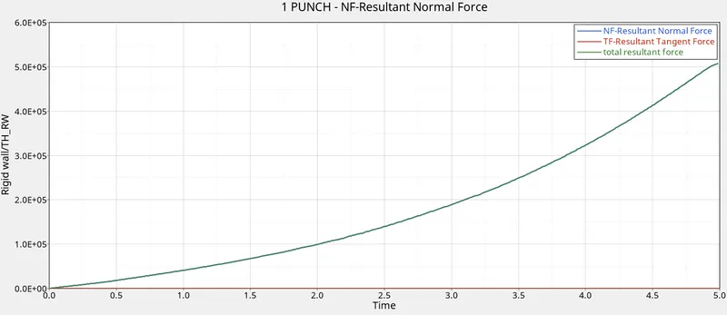
  The rate of increase of magnitudes in both the plots goes on increasing as the simulation progresses.
  This is due to the fact that an elastic material develops higher and higher stresses as the deformation progresses since there is no scope for permanent deformation here.
  
  
• The energy error and mass error values at the end are 1.9% and 0.00 respectively.
  
  
  
  
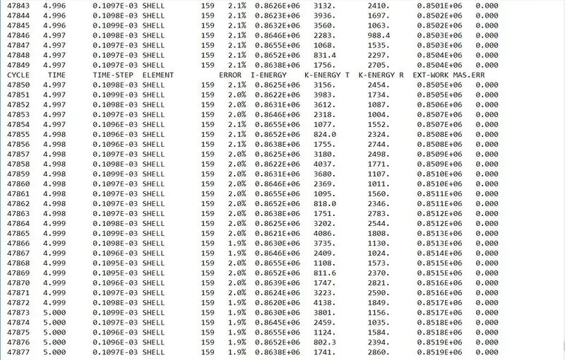
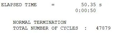
• The simulation time and number of cycles occured is shown below.
  

Case VI : To change the shell properties to recommended values in the provided LAW27 file and run the mode with name LAW27.

• The provided Law27 file is imported in HyperMesh.
• The Law27 material card essentially combines a Johnson-Cook material card with an Orthographic Brittle material card.
• This is typically suited for brittle materials such as the car windshields, etc.
• One thing to notice here is this card only accounts for the tensile failures.
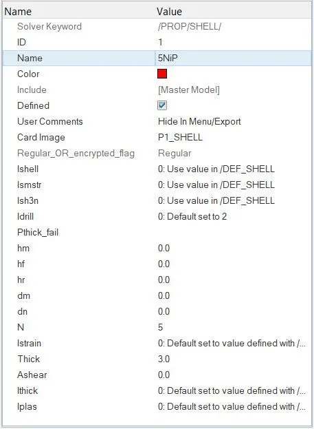
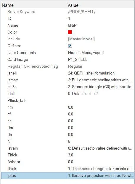
• Here, the default property card flags are changed to the recommended shell property flags as shown below.
  
  
  
  
• The material properties and flag values are left with their default values.
  
  
  
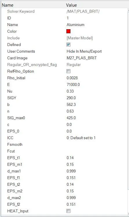
  The material properties in this case are much similar to that of the Johnson card with additional terms such as EPS_t, EPS_m, d_max, EPS_f which correspond to the points of tensile failure and element deletion.
• The value of d_max (maximum damage factor) governs the time period between the tensilee failure and actual failure.
  The more the value of d_max leaning towards 1, the higher will be the rate at which the stress in the material falls to zero.
• These terms basically define the stress-strain relationship of the brittle material over the working range.
  The plastic behaviour region is very small in this case as it is for a brittle material.
  
  
• Then model is exported with the name Law27 and ran for simulation.
  
  

Results :

• By running the H3D file. the plate failure can be analysed.
  
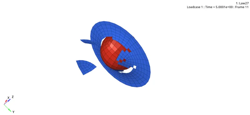
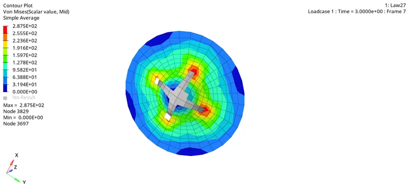
• The von mises stress contour is shown below (maximum value being 287.5 MPa)
  
  
  
  
• The plots of energies and rigid wall forces show similar behaviour as seen in the cases 1 and 2.
  
  
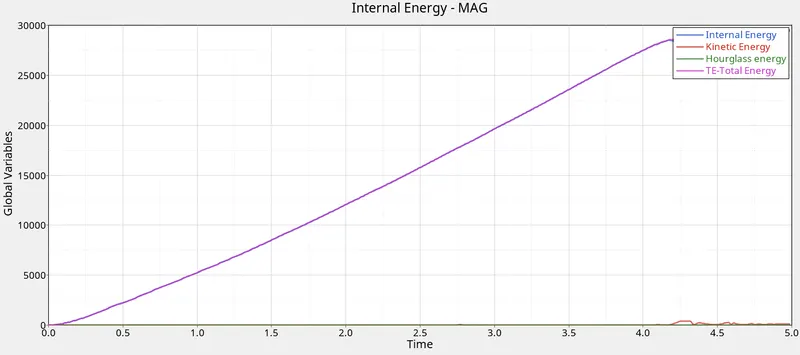
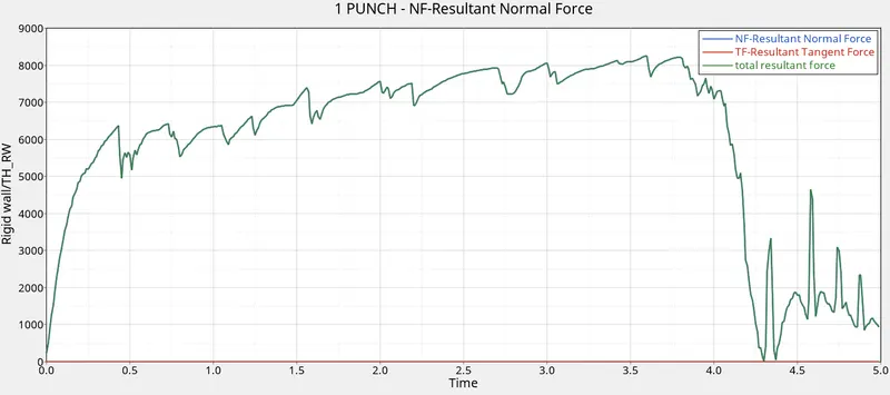
  Due to the deletion of elements over the simulation run, the force graph shows a fluctuating behaviour.
  
  
• The energy error is as low as 0.9% with no mass error at the end of simulation.
  
  
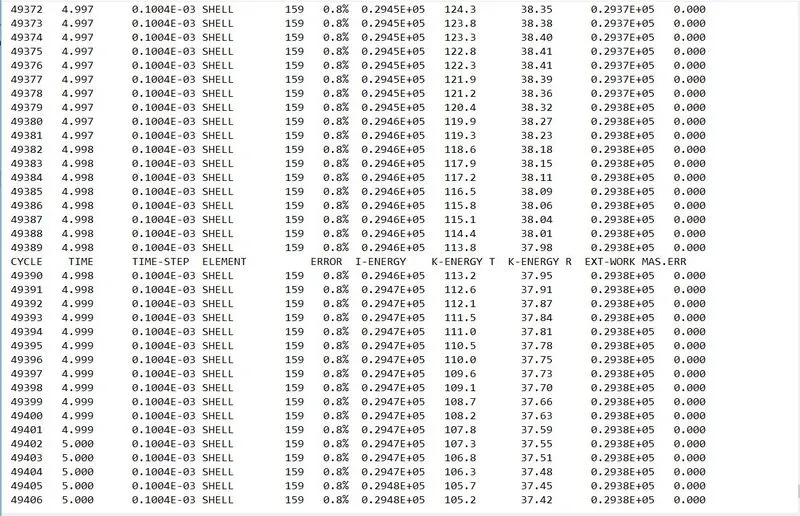
• The simulation time and number of cycles elapsed are shown below
  
  

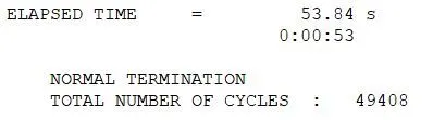
Case VII : To convert the card to Law36 elastoplastic material as per the recommended properties.

• Law36 card corresponds to the PLAS_TAB (piecewise linear) material card wherein the material behaves in elasto-plastic manner.
• This card is the most widely used in industrial applications.
  
  
• To formulate this card, parameters are needed, which define a function which directly corresponds to the stress-strain behaviour of the material beyond the yield point.
• Such a function is first created using the Curve card.
  
  
  
  
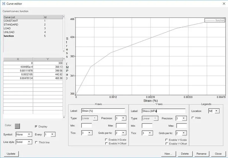
• This function is now assigned inside the material card.
  The new material card is shown below -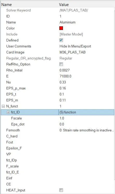
  
  
  
  Here, the material properties such as E, rho and nu are left with their previous values.
• The model is now ran for simulation.

Results :

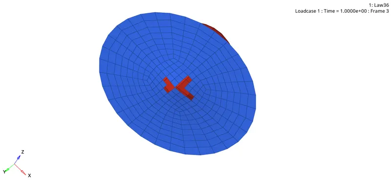
• The failure start in this case is slightly different.
  
  
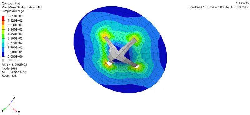
• Von Mises stress contour is shown below
  
  
  
• Plots of energies and rigid wall forces -
  
  
  
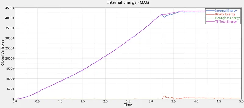
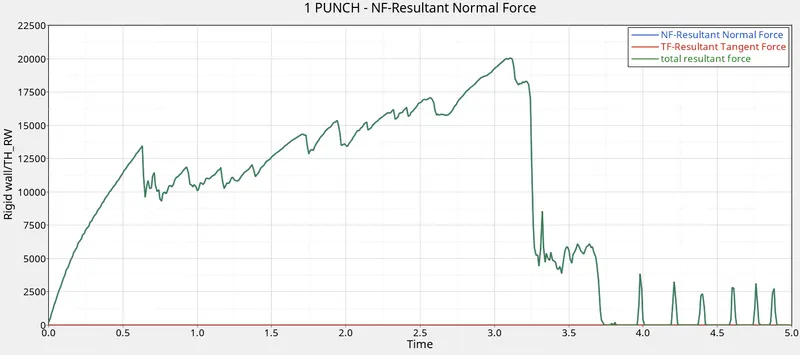
  Here, the energy plot shows the constant behaviour very early than the earlier cases indicating that the ball has penetrated the plate at this instant.
  The wall forces plot shows a similar behaviour as well.
  
  
• The energy error in this case is -1.5 at the simulation end i.e. negative, which is the most desired case. Also, the magnitude of it is much below that of the allowed limit (5%).
  
  
  
  
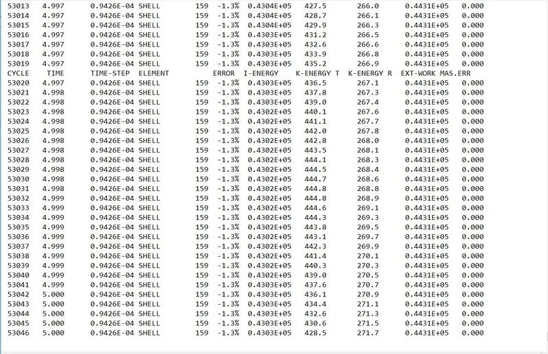
• Elapsed time and the total number of cycles -
  
  
  
  

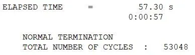
CONCLUSION :

Succesfully ran the simulations for all the 7 cases and analysed the results.

Judging by the nature and amount of energy errors generated in each individual case, the Law36 card must be the best suited card for on-field scenarios.
Also, the card corresponds to the elasto-plastic behaviour of the material wherein the elastic zone is characterized by the material properties such as E,rho and nu. Similarly, the plastic region is defined by the curve function values.
This results in effective analysis of the material throughout the working region.

I also learnt quite a lot of interesting things such as -

1. What are the different types of material cards which can be used in impact analysis.
2. What is elasto-plastic material card and what are its advantages.
3. How each card is different from the others and under what conditions is it best suitable.
4. How to properly analyze the results in HyperView and HyperGraph windows.