Wide Open Throttle (WOT) condition of GM EV1 car

AIM :

1. To calculate the ratio of hill-climbing power required by fully loaded tata ultra truck to the half-loaded one.
2. To calculate the minimum length of the flyover, considering the minimum height at the summit should be 5.5 meters
3. To prepare a new drive cycle excel file for the model and also include a hill-climbing angle to it. Also, revise the model file “Driver_Glider.slx” and comment on the results
   https://in.mathworks.com/matlabcentral/fileexchange/63823-matlab-and-simulink-racing-lounge-vehicle-modeling
4. To model the WOT (Wide Open Throttle) response of GM EV1 car and compare it with the official figures of the performance of a real vehicle. Also, to prepare a table showing variation in acceleration time with a 5% change in vehicle parameters.

SOLUTION :

(1) - To calculate the ratio of hill-climbing power required by fully loaded tata ultra truck to the half-loaded one.

The TATA 10 tonner ULTRA truck is considered for the study (ULTRA 1012).

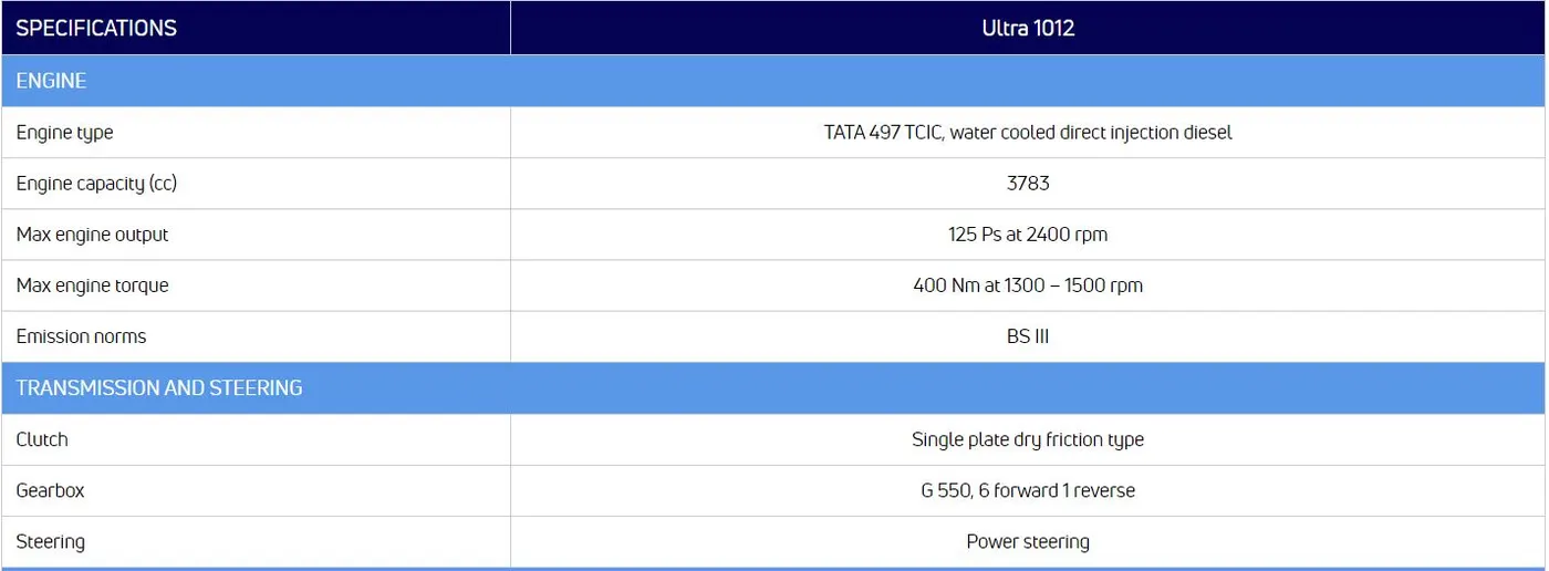
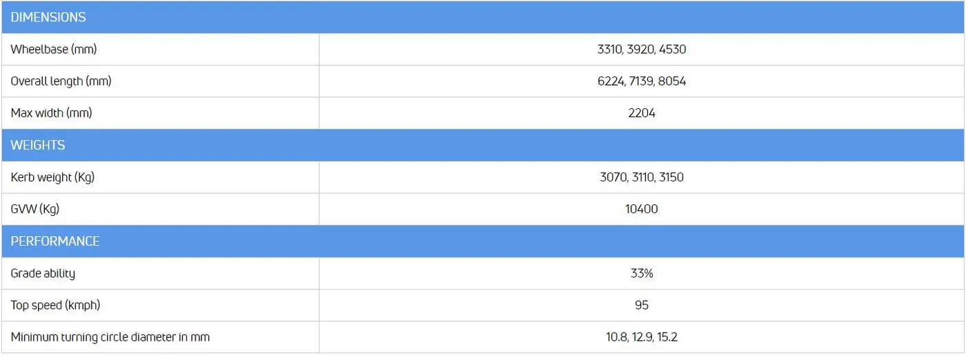
Here,

Kerb Weight = 3150kg

GVW (Gross Vehicle Weight) = 10400 kg = Kerb weight + Payload
∴ Payload 1 = 10400 - 3150 = 7250 kg ..... [fully loaded condition]
& Payload 2 = 7250/2 = 3625 kg ..... [half loaded condition]

Gradeability = 33% = 18.26°

We know, the hill climbing force acting on a vehicle, Fhc=m⋅g⋅sinα

& the hill climbing power reqd. by a vehicle, Phc=Fhc⋅v

Where,

m = kerb weight + payload
g = gravitational acceleration = 9.81 m/s2
α= grade angle (inclination of road)
v = velocity of vehicle (m/s)

∴ m1 (fully loaded) = 3150 + 7250 = 10400 kg
m2 (half loaded) = 3150 + 3625 = 6775 kg

∴ Ratio of hill climbing power reqd. in the two cases = Fhc1/Fhc2
= m1/m2 .... [rest all parameters are same in both cases]
= `10400/6775`
= 1.535

Result : The ratio of hill-climbing power required by fully loaded tata ultra truck to the half-loaded one = 1.535

(2) - To calculate the minimum length of the flyover, considering the minimum height at the summit should be 5.5 meters

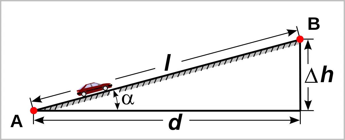
Here,
for TATA ULTRA 1012, gradeability = 33%

∴ α= 18.26°

∴ sinα=h/l

where,
h = rise of the flyover = 5.5 m (given)
l = length of the flyover

∴ l=hsinα
= 5.5sin18.26
= 17.55 m

Result : The minimum length of the flyover is 17.55 m

(3) - To prepare a new drive cycle excel file for the model and also include a hill-climbing angle to it. Also, revise the model file “Driver_Glider.slx” and comment on the results

Driver Glider model :

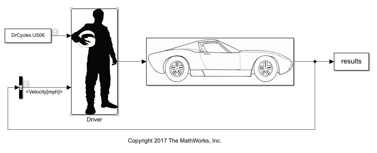
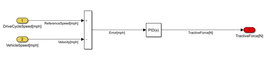
Driver subsystem :

Glider Subsystem :

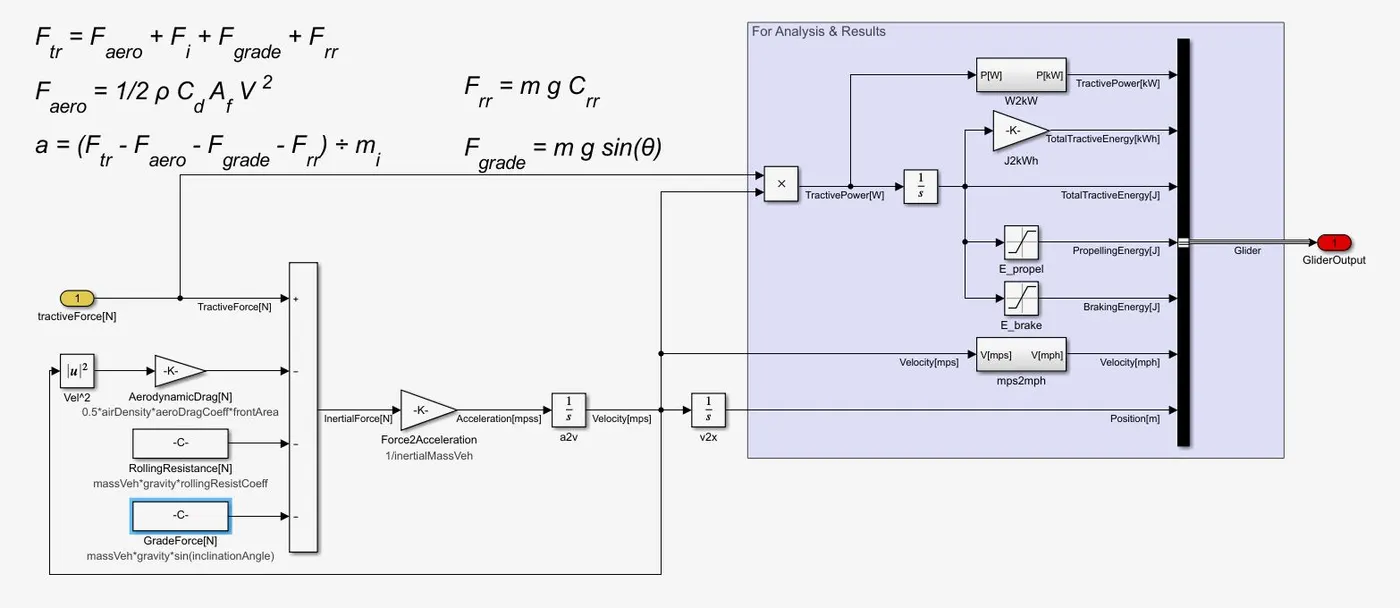
• The glider subsystem takes input parameters such as Drag coefficient, Rolling Resistance and Grade angle and with the help of proper mathematical modeliing, gives out the Glider Output.
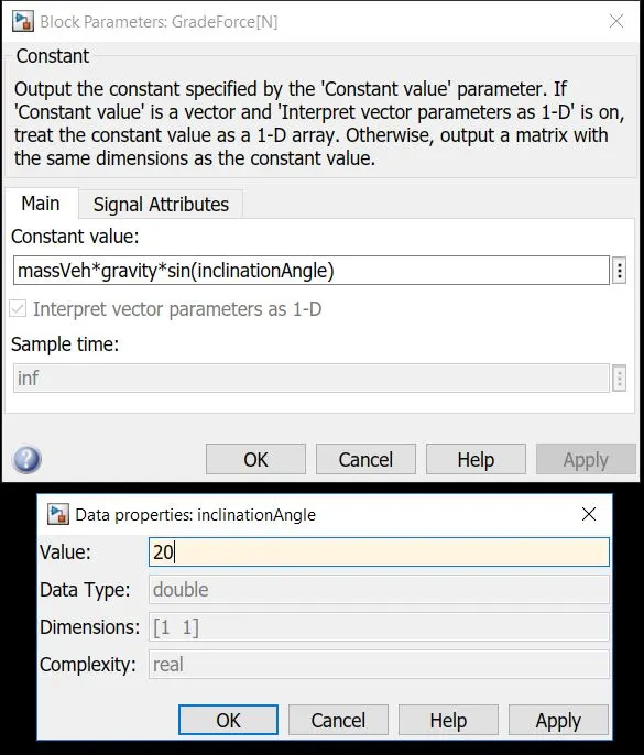
• Here, initially no road inclination is considered. The grade angle can be changed from the model workspace of the GradeForce block.
  
  
  
  
• To create a new Drive cycle, an Excel Spreadsheet is created. It consists of two columns (Time and Velocity in mph). The time values are kept as integer values from 0-500, while random values are added as the corresponding velocity values.
  The spreadsheet file with the name 'NewDrivingCycle' is attached with the report for reference.
• Now, this file is to be imported into the Base Workspace. For this, the Import command from the upper command ribbon is used. The output type is chosen as Numeric Matrix.
  
  
  
  
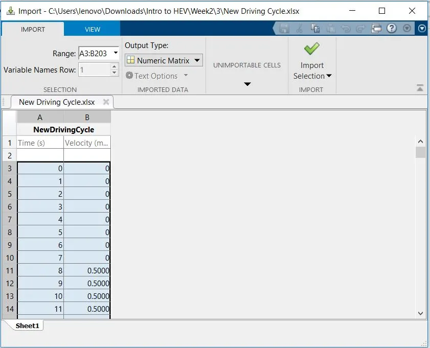
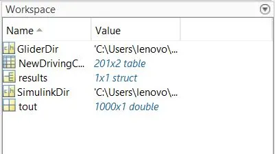
• This file can now be used as a Drive Cycle in the Simulink model with the help of From Workspace block.
  
  

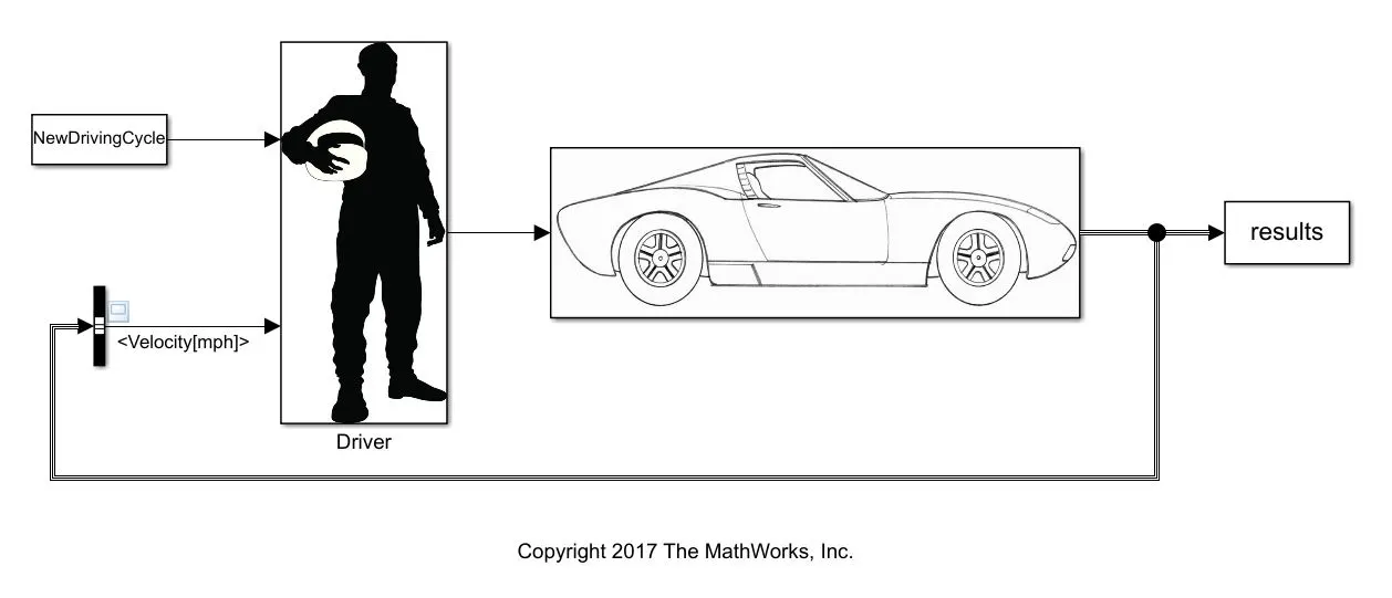
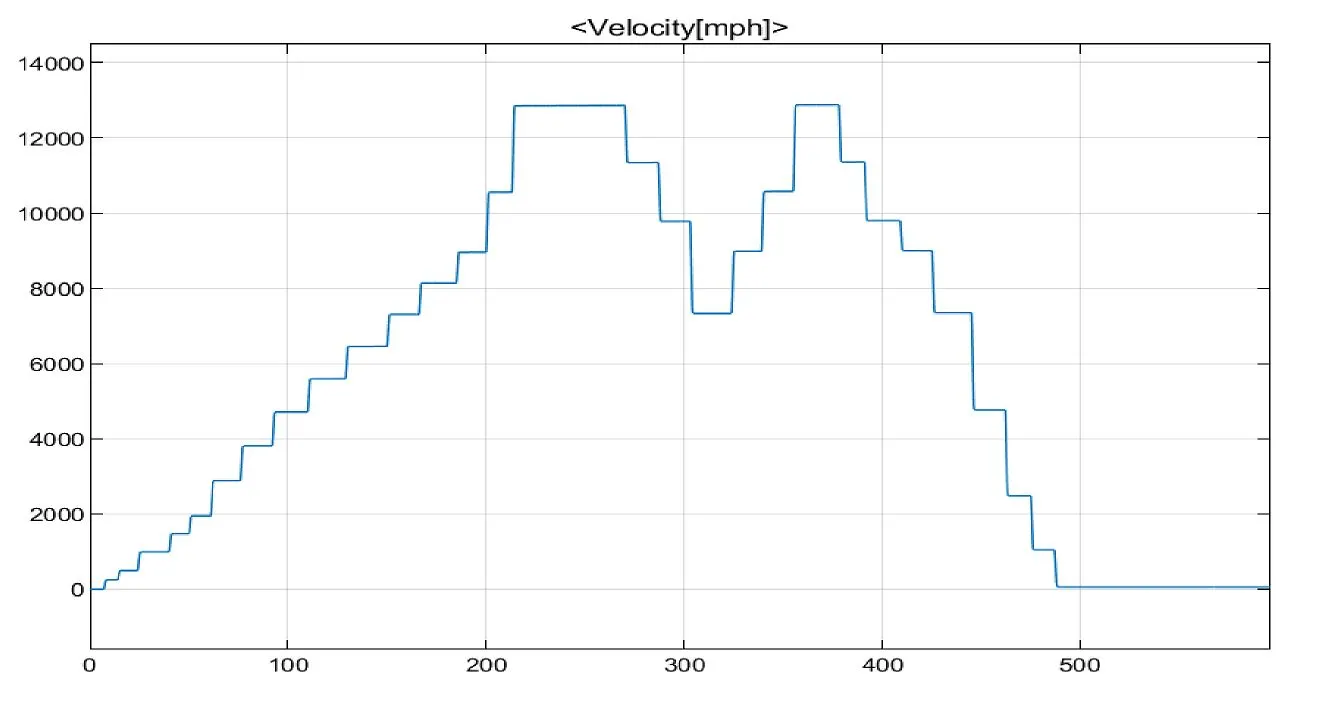
Result/Output :

• The model is now run for simulation and the output is observed.
  
  
  
  
  

(4) - To model the WOT (Wide Open Throttle) response of GM EV1 car and compare it with the official figures of the performance of a real vehicle. Also, to prepare a table showing variation in acceleration time with a 5% change in vehicle parameters.

The General Motors EV1 was an electric car produced and leased by General Motors from 1996 to 1999. It was the first mass-produced and purpose-designed electric vehicle of the modern era from a major automaker and the first GM car designed to be an electric vehicle from the outset.

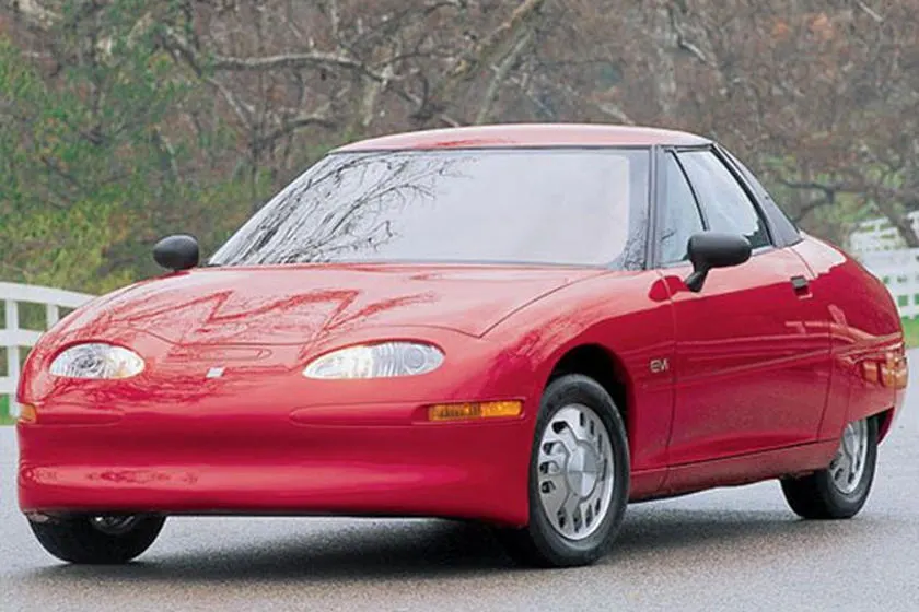
Wide Open Throttle : The WOT condition is nothing but the high acceleration case, wherein the vehicle (initially at rest) starts accelerating and tries to reach its top speed when the driver applies full throttle within a small interval of time.

To study this Wide Open throttle condition of the car, the following fundamental equation is used -

`G/rT = mu*m*g+0.5*rho*A*Cd*v^2+(m+IG^2/(eta*r^2))(dv)/dt`

where,

G = gear ratio
r = radius of wheels
T = Torque required by wheels
mu = coefficient of rolling resistance
m = total mass of vehicle
g = gravitational acceleration = 9.81 `m/s^2`
rho = density of surrounding fluid (for air = 1.25 `(kg)/m^3`
A = frontal area of the vehicle
Cd = drag coefficient
v = velocity of the vehicle
I = moment of Inertia of rotating parts
η= gear box efficiency
t = time

This equation can be modified a bit if the surrounding fluid is air -

`G/rT = mu*m*g+0.625*A*Cd*v^2+(m+IG^2/(eta*r^2))(dv)/dt`

Here are some specifications of GM EV1 -

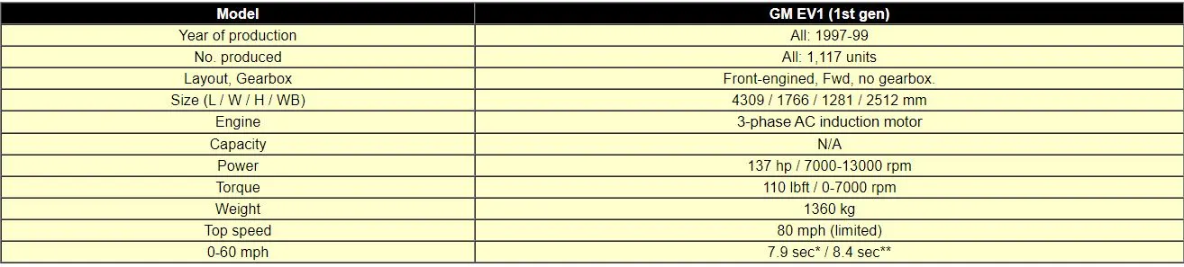
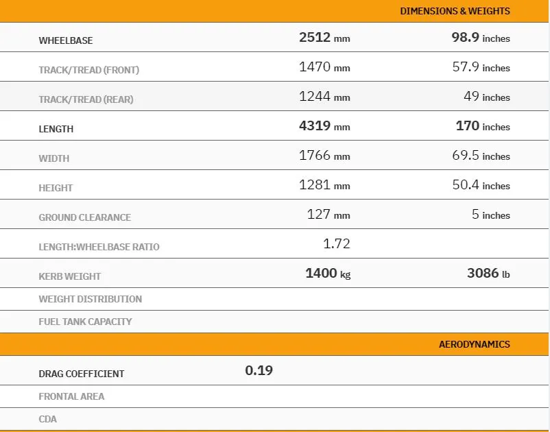
Let us analyse the WOT condition for the car based on some assumptions of our own -

Gross weight of vehicle = 1540 kg ....[assuming Kerb Weight =1400 kg & additioanl 140 kg for passengers]
Since, comapred to the vehicle mass, the rotor masses are very less, the total mass of the vehicle can be approximated to 1560 kg
Drag coefficient = 0.19 ....[since the GM EV1 has nearly perfect streamlined body]
Coefficient of rolling resistance = 0.0048
Gear Ratio = 11
`eta`= 95 %
Wheel radius = 0.3 m
Frontal Area = 1.8 m^2
Tmax of motor = 140 Nm
Critical angular speed of motor = 733 rad/s ; ....[corresponding v =19.8 m/s]
Above critical speed, motor operates at constant power of 102 kW

Top speed = 80mph .... [from above mentioned speecifications]
= 35.7 m/s

Now, until critical speed is reached, the motor operates at a constant Torque i.e Tmax

Case I : for ω≤ωc

by subsituting the above values in the fundamental equation, we get,

`(dv)/dt = 3.11 - 0.000137v^2`

this differential equation can be written in the 'finite difference' form as -

Vn+1=Vn+∂t(3.11-0.000137v^2)

Case II : Similarly, for ω>ωc ....[Power = constant ; ∴ T=P/v]

we get -

Vn+1=Vn+∂t(62.1/v-0.046-0.000137v^2)

The equations are solved in MATLAB -

clear all
clc

t = linspace(0,50,501);                 %creating time array with 0.1s incremental value
v = zeros(1,501);                       %initially creating a zero array for velocity 
d = zeros(1,501);                       %initially creating a zero array for distance covered  
dt = 0.1;

for n=1:500
    if v(n) <= 19.8;
        v(n+1) = v(n) + dt*(3.11 - 0.000137*(v(n)^2));
    else if v(n) > 19.8;
            v(n+1) = v(n) + dt*((62.1/v(n)) - 0.046 -0.000137*(v(n)^2));
        end
        if v(n) >= 35.7
            v(n+1) = v(n)                    %top speed
        end
    end
    d(n+1) = d(n) + 0.1*v(n);
end

v = v.*(3.6);                                %converting into kmph
d = d.*0.001;                                %converting into km

%plotting the curve
figure(1)
subplot(2,1,1)
hold on
plot(t,v);
xlabel('Time (sec)');
ylabel('Velocity (kmph)');
grid on
subplot(2,1,2)
plot(t,d);
xlabel('Time (sec)');
ylabel('distance (km)');
grid on

• Initially, 2 zero arrays are created for values of velocities and distances. These values are overwritten as the program executes further.
• The numerical equations are run inside a for loop to get 500 values of v and d.
  Accordingly, if v<=19.8, the first equation is executed. If v>19.8 but <35.7, the second equation comes into play. Above the top speed i.e 35.7m/s, the velocity remains constant.
• Plots are generated to visualise the outputs.
• The code file is attached with the report for reference.
  
  

Result/Output :

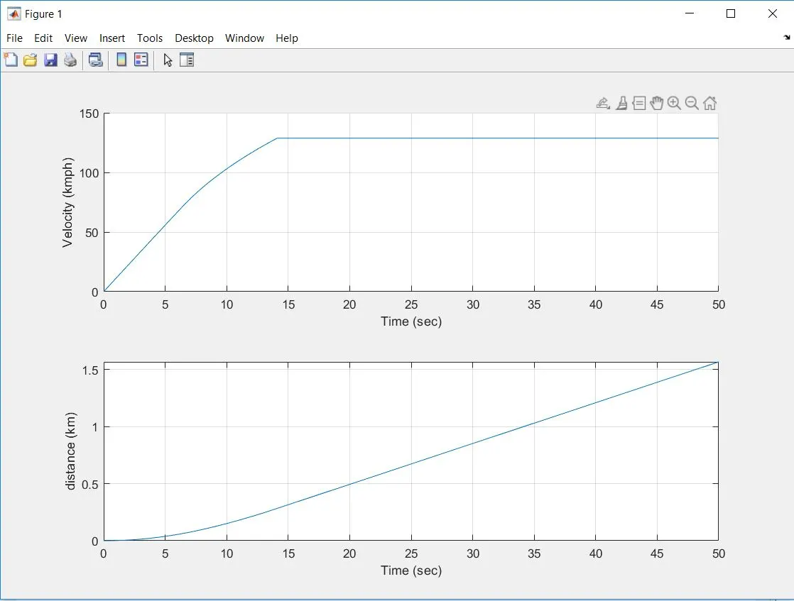
• The vehicle reaches its top speed (35.7 m/s or 129.6 kmph) in about 14 sec.
• The corresponding distance covered before reaching the top speed is nearly 0.3 km.

Comparing this result with the performance of a real vehicle :

Actual Vehicle performance : (taken from the internet)

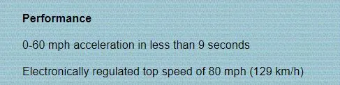
From the results of our analysis, the vehicle reaches 60 mph i.e 96.5 kmph in almost 9 sec. (From the above mentioned plot).

This means, our analysis is very much accurate and the result data matches with the actual vehicle specifications.

# Now, let us change some of the vehicle paramaters by 5% of the initial values. Hence, the new values are -

Total mass of vehicle = 1638 kg
Coefficient of rolling resistance = 0.005
Frontal Area = 1.89 m^2
Wheel radius = 0.315

The new equations are -

for v<=19.8 m/s : dv/dt=2.78-0.000137v^2

for v> 19.8 m/s : dv/dt=55.7/v-0.048-0.000137v^2

The equations are solved with the similar code as above, in MATLAB -

clear all
clc

t = linspace(0,50,501);                 %creating time array with 0.1s incremental value
v = zeros(1,501);                       %initially creating a zero array for velocity 
d = zeros(1,501);                       %initially creating a zero array for distance covered  
dt = 0.1;

for n=1:500
    if v(n) <= 19.8;
        v(n+1) = v(n) + dt*(2.78 - 0.000137*(v(n)^2));
    else if v(n) > 19.8;
            v(n+1) = v(n) + dt*((55.7/v(n)) - 0.048 -0.000137*(v(n)^2));
        end
        if v(n) >= 35.7
            v(n+1) = v(n)                    %top speed
        end
    end
    d(n+1) = d(n) + 0.1*v(n);
end

v = v.*(3.6);                                %converting into kmph
d = d.*0.001;                                %converting into km

%plotting the curve
figure(1)
subplot(2,1,1)
hold on
plot(t,v);
xlabel('Time (sec)');
ylabel('Velocity (kmph)');
grid on
subplot(2,1,2)
plot(t,d);
xlabel('Time (sec)');
ylabel('distance (km)');
grid on

Result/Output :

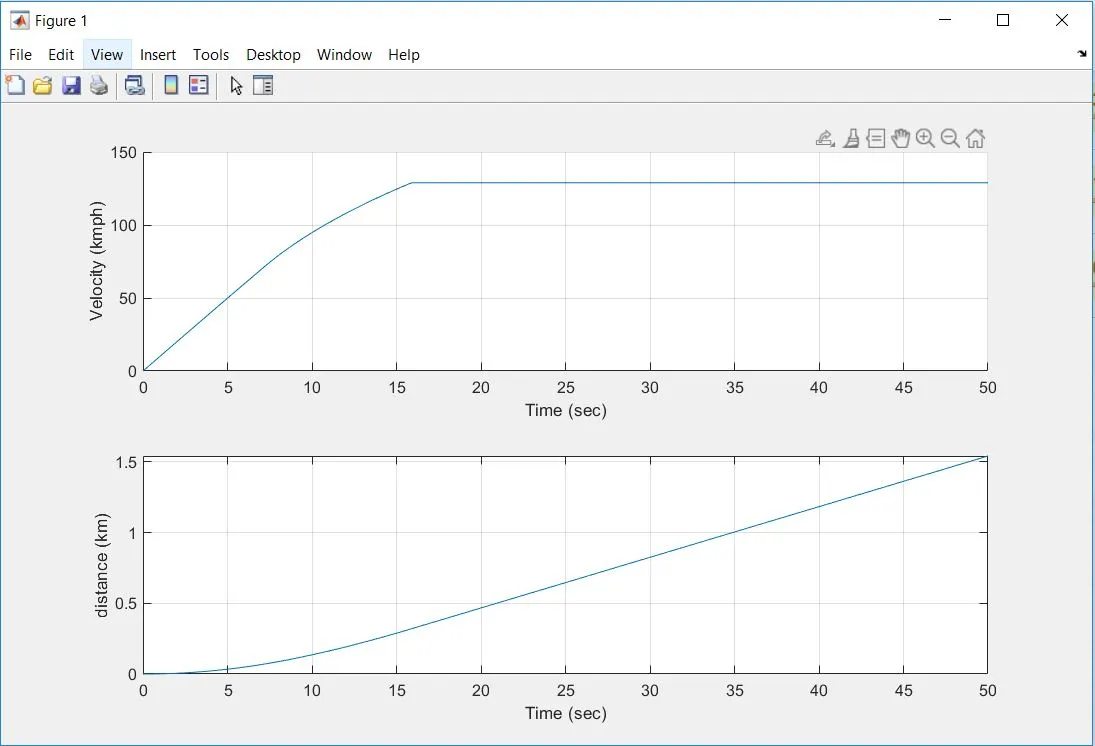
• In this case, the the vehicle runs for about 16 sec before reaching the top speed.
• The corresponding distance covered is 0.35 km

CONCLUSION :

1. The ratio of hill-climbing power required by fully loaded TATA ULTRA 1012 truck to the half-loaded one comes out to be 1.535
2. the minimum length of the flyover for the appropriate gradeability is 17.55 m
3. The Driver Glider model is simulated with our own drive cycle and assumed value of grade angle.
4. (a) The analysis done by us is accurate and the performance matches with the actual vehicle performance.
   (b) The WOT time or the acceleration time taken by the vehicle to reach its top speed increases by about 2 sec when the vehicle parameter values are increased by 5%.