Week 9 - FVM Literature Review
What is The Finite Volume Method:
The FVM is a discretization method for the approximation of a single or a system of partial differential equations expressing the conservation, or balance, of one or more quantities.These PDEs are used as models in a wide number of fields and they are indifferent natures such as parabolic, hyperbolic and elliptic. They are also used to describe the relations between partial derivatives of unknown fields such as Temperature, Pressure, Velocity, density, molar fraction, and so on only under certain considerations
As in the finite element method, a mesh is constructed, which consists of a partition of the domain where the space variable lives. The elements of the mesh are called control volumes. The integration of the PDE over each control volume results in a balanced equation. The set of balance equations is then discretized with respect to a set of discrete unknowns. The main issue is the discretization of the fluxes at the boundaries of each control volume: in order for the FVM to be efficient, the numerical fluxes are generally *conservative and *consistent.
*Conservative means the flux entering a control volume from its neighbor must be the opposite of the entering the neighbor from the control volume.
*Consistent means the numerical flux of a regular function interpolation tends to the continuous flux as the mesh size vanishes.
Finite volume refers to the small volume surrounding each node point on a mesh. In FVM equations are written in an entire volume and no assumptions were made over the shape of the volume. Inside this particular volume, all the flow quantities are conserved.
Types of FVM grids: The grids are again divided into two types structured and unstructured grids.
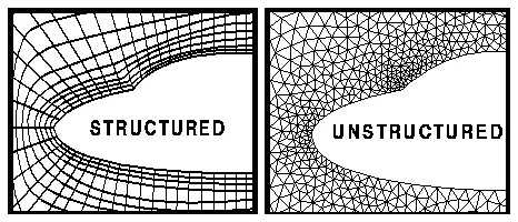
Cell centred approach: control volumes are defined by a suitable grid and computational nodes are assigned at the control volume centre. It can be applied for both structured and unstructured grids. Cell centred nodal values represent mean over the control volume. This approach is the most commonly used in the Finite Volume Method- Face centred approach: Nodal locations are defined first and control volumes are then constructed around them so that the control volume faces lies in the nodal points. It can only be used with structured grids.
- Approximation of surface integral: Net flux through the control volume boundaries is the sum of the integral over the control volume faces. where 'f' is the component of the convective or diffusive flux in the direction normal to the control volume.
`int_s f ds= sum_k int_(s_k) f ds`
Steps in Discretizing the Finite Volume Method:
First, obtain the governing equations.
Second apply the solvers
Third choose a suitable method for calculating the flux terms
`del/(delX)(alpha(delT)/(delX))+s=0`
S is the source term
`(delT)/(delX)` is the temperature gradient along x-direction
`alpha` is the Thermal diffusivity
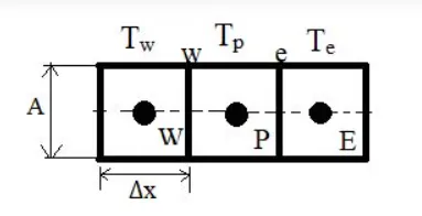
The governing equations are valid at every point in the domain which means it is valid in the entires control volume
Now we multiply the governing equation with dv and integrating it
`int((del)/(delx)(alpha(delT)/(delx))+s)dv=0`
`int(del)/(delx)(alpha(delT)/(delx))dv+ints dv=0`
dv=A*dx
`int_w^e(del)/(delx)(alpha(delT)/(delx))Adx+ints dv=0`
`[alphaA((delT)/(delx))]_w^e+barsdv=0`
`barS` is the average value of the source term(s)
`[alpha_eA((delT)/(delx_e))]-[alpha_wA(delT)/(delx_w)]+barsdv=0`
heat flux out - heat flux in + `s_u+s_pT_p`
`alphaA[(T_e-T_p)/(trianglex)]-alphaA[(T_p-T_w)/(trianglex)]+barsdv=0`
The main difference between FDM and FVM:
A finite difference method (FDM) discretization is based upon the differential form of the PDE to be solved. Each derivative is replaced with an approximate difference formula which can usually be derived using Taylor series expansion. The computational domain is usually divided into hexahedral cells(the grid), and the solution will be obtained at each nodal point. The FDM is easiest to understand when the physical grid is Cartesian, but through the use of curvilinear transforms the method can be extended to domains that are not easily represented by brick-shaped elements. The discretization results in a system of the equation of the variable at nodal points, and once a solution is found, then we have a discrete representation of the solution.
A finite volume method (FVM) discretization is based upon an integral form of PDE to be solved for example conservation of mass, momentum, and energy. The PDE is written in a form that can be solved for a given finite volume (or cell). The computational domain is discretized into finite volumes and then for every volume, the governing equations are solved. The resulting system of equations usually involves fluxes of the conserved variable, and thus the calculation of fluxes is very important in FVM. The basic advantage of this method over FDM is it does not require the use of structured grids, and the effort to convert the given mesh into a structured numerical grid internally is completely avoided. As with FDM, the resulting approximation solution is discrete, but the variables are typically placed at cell centers rather than at nodal points. This is not always true, as there are also face-centered finite volume methods. In any case, the values of field variables at non-storage locations are obtained using interpolation.
Necessary of Interpolation Schemes in Finite Volume Method:
The approximation of surface and volume integrals may require values of the variable at locations other than the computational nodes of the CV. Values at these locations are obtained using interpolation formulae. Some of the possibilities are:
Upwind Interpolation Scheme(UDS)
The name upwind refers to the assumptions that we are going to use the node that is upwind or upstream of the given node. It is generally used for convection dominated problems(i.e. High Peclet Number Pe>1 flows). For the east face of a quantity, it is given as
`f_e={(,f_e if,(v.n)_e,>,0),(,f_E if,(v.n)_e,<,0):}`
`(v.n)_e` is the velocity component at point e in the x-direction.
These interfaces are also given by
for v>0, we have `ui - 12 ~~ ui - 1; ui +12 ~~ ui`
`Ic ~~ v(ui-ui-1)/(triangle)x` (Backward Differencing)
for v<0, we have `ui - 12 ~~ ui; ui +12~~ ui+1`
`Ic~~v(ui+1-ui)/(triangle)x` (Forward Differencing)
The above two differencing schemes are part of taylor series.
Advantages: This scheme satisfies the boundedness criterion, in the sense that irrespective of velocity values and the grid spacing solution
Disadvantages: This scheme is numerically diffusive, the rapid variations in the variables will be streaked out.
Linear Interpolation Scheme: it is the simplest and most widely used interpolation. In this case, we approximate the values of the variable at Control Volumes face center by interpolating the values linearly at the two nearest computational nodes. The linear interpolation is equivalent to the use of the central difference formula of the first order derivative and hence it is also called as Central Difference Scheme.
`f_e=f_Elamda_e +f_p(1-lamda_e)` `lamda_e=(X_e-X_p)/(X_E-X_p)`
`lamda_e` is the function of the computational nodes E and P with respect to eastern face.
Quadratic upwind interpolation: In this case we have to approximate the value of the variable at control volume face centre by quadratic interpolation of the values at three nearest computational nodes
`f_e=f_u+g_1(f_D-f_U)+g_2(f_(UU)-f_U)`
`g_1=((X_e-X_u)(X_e-X_(U U)))/((X_D-X_U)(X_D-X_(U U)))`
`g_2=((X_e-X_u)(X_e-X_D))/((X_(U U) -X_U)(X_(U U) - X_D))`
Hybrid Scheme:
This scheme is the combination of Upwind interpolation scheme and central distribution scheme based on the local peclet number.
`f_e=gammaf_(cds)+(1-gamma)f_(cds)`
Total Variation Diminsh:
`f_e=f_p+0.5**psi**r**(f_e-f_p)`
`psi` is a local flux limiter
r is a function dependent on the local flow conditions.
Flux Limiter's: They are used in high resolution schemes numerical schemes used to solve problems in engineering, particularly fluid dynamics, described by partial differential equations. They are used in high resolution schemes, such as the MUSCL scheme, to avoid the spurious oscillation. This could occur with high order spatial discretization schemes due to shocks, discontinuity or sharp changes in the solution domain. Use of flux limiters, together with an appropriate high resolution scheme, make the solutions Total Variation Diminishing(TVD).
Note that flux limiters are also referred to as slope limiters because they both have the same mathematical form, and both have the effect of limiting the solution gradient near shocks or discontinuities. In general, the term flux limiter is used when the limiter acts in systems fluxes, and slope limiter is used when the limiter acts on system states like pressure, velocity, temperature.
How actually they work: The amin ides behind the construction of flux limiter schemes is to limit the spatial derivatives to realistic values- for scientific and engineering problems this usually means physically realisable and meaningful values. they are used in high resolution schemes for solving problems describes by PDEs and only come into operation when sharp wave fronts are present. For smoothly changing waves, the flux limiters do not operate and the spatial derivatives can be represented by higher order approximations without introducing spurious oscillations.
Consider 1D linear heat conduction equation:
For one-dimensional heat conduction (temperature depending on one variable only), we can devise a basic description of the process. The first law in control volume from (steady flow energy equation) with no shaft work and no mass flow reduces to the statement that `sumdotQ`for all surfaces = 0(no heat transfer on top or bottom of above picture)
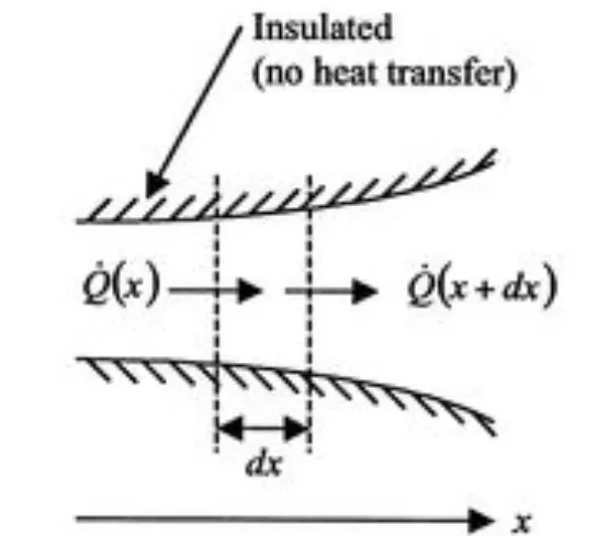
The heat transfer rate from left at x
`Q(x)=-k(A(dT)/(dx))_x`
here the negative sign indicates that heat flow down the temperature gradient.
The heat transfer rate on the right
`Q(x+dx)=Q(x)+(dQ)/(dx)|_x`dx+...
Using the conditions on the overall heatflow and the expressions
`Q(x)-(Q(x)+(dQ)/(dx)(x)dx+...)=0.`
Taking the limit as dx approaches zero we obtain
`d/(dx)(kA(dT)/(dx))=0`