Week 4.1: Project - Steady state simulation of flow over a throttle body

AIM: The main objective of this challenge is to simulate a steady-state fluid flow through an elbow-shaped pipe with a throttle valve inside it.

INTRODUCTION: The simulation was performed on a given geometry. There are a few modifications to be done to the model.

1. Firstly, removing the thickness.
2. Lastly, closing the open surfaces or boundaries.

      

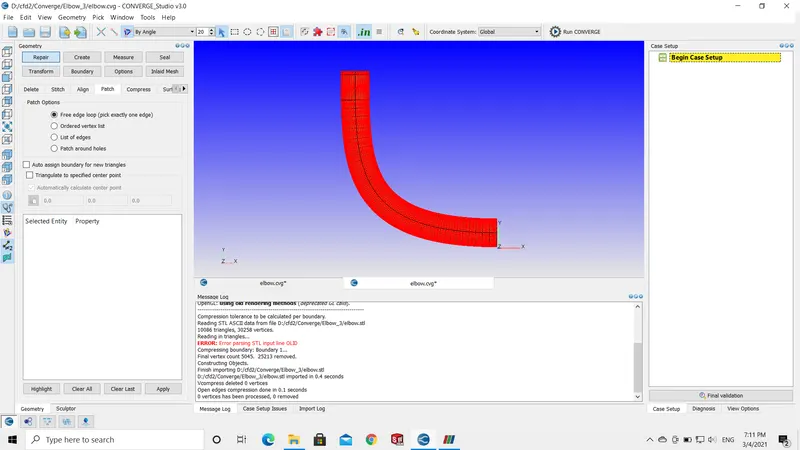
• The aim of the simulation is to study the characteristics of fluid through the elbow, not the Conjugate Heat Transfer(CHT) through the wall. Select the outer surface using the "By Angle" option and press D to delete the surface. By using this method, delete the extra layers or thickness on the pipe.
• After completing the above process, close the openings on either side of the pipe using the Repair --> Patch option. Lastly, the geometry looks as below.

THEORY:

• Before getting started with the case setup, make sure the geometry has zero errors and flag the boundary.
• In this type, we have parts inside the geometry (throttle valve) make sure to flag them properly using the "By Surface" option.
• Start the case setup, it is a time-based application.
• The material flowing inside the geometry is air (23% O2 and 77% N2).

CASE SETUP:

• MATERIALS: The fluid inside will be air.
• The global transport parameters will have default values.
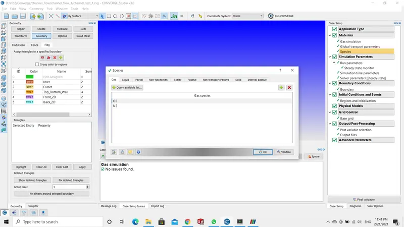
• Species: as the fluid inside the pipe, is air add O2 and N2 variables.

        

        

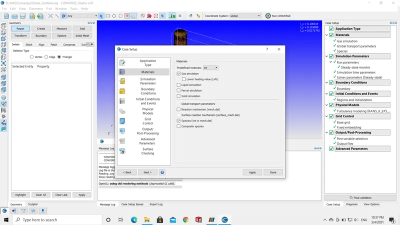
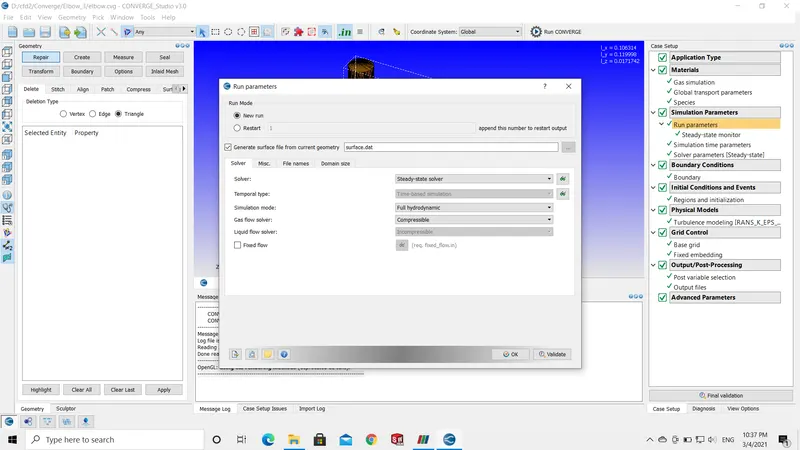
• SIMULATION PARAMETERS: It includes the type of solver used and the duration of the parameter.
• Run Parameter: Steady-State type of solver is used for this simulation.
• In run parameter next to solver tab i.e in MISC section uncheck the use shared memory and enable the steady-state monitor.
• In steady-state monitor include the parameter you are intended to see. In this case, the mass flow rate at the output is being calculated.
• Simulation Time Parameter: The case is being calculated for 15000 cycles the CFL number is 1 and in the Solver Parameter the maximum CFL number should be 0.5 i.e less than the value mentioned in the simulation parameter.
• In the solver parameter, the Navier-Stokes parameter should be Density-Based. 

      

      

       

         

      

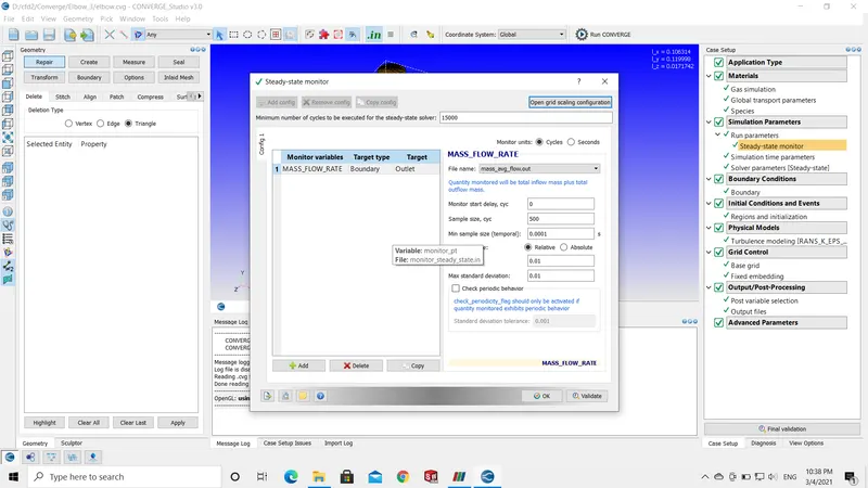
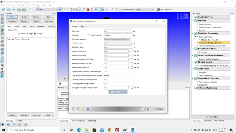
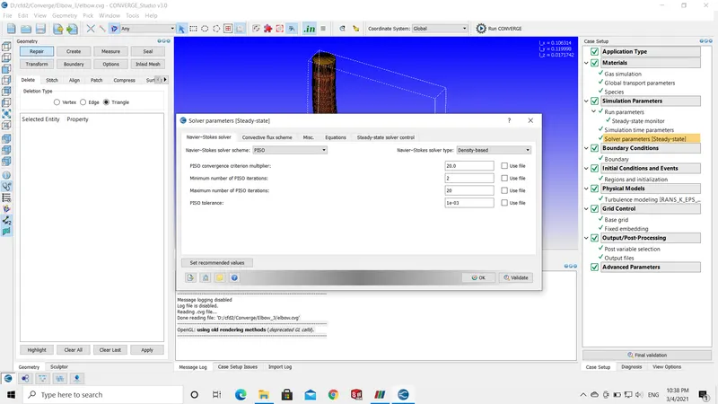
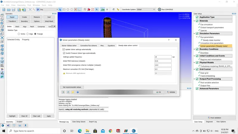
• BOUNDARY CONDITIONS AND REGIONS & INITIALIZATION:
• Both the boundary conditions and region setup are interlinked. In regions and initializations, the pressure or velocity, temperature and type of fluid are described. Whereas in boundary conditions the geometrical model boundaries are flagged and to every condition, the regions are assigned.
• The inlet pressure is 150000 Pa.
• The outlet pressure is 100000Pa. 

        

        

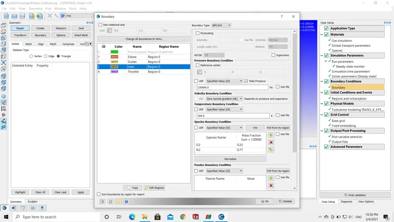
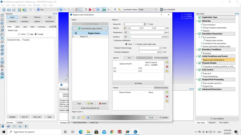
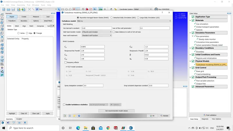
• PHYSICAL MODEL:  This is a turbulence viscous flow. RANS k-epsilon model is implemented for this.

        

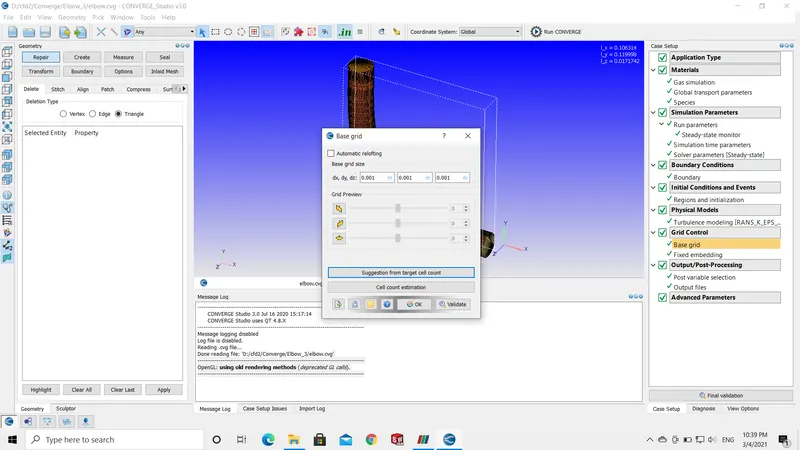
• GRID CONTROL: 
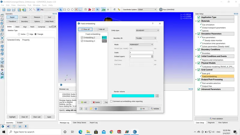
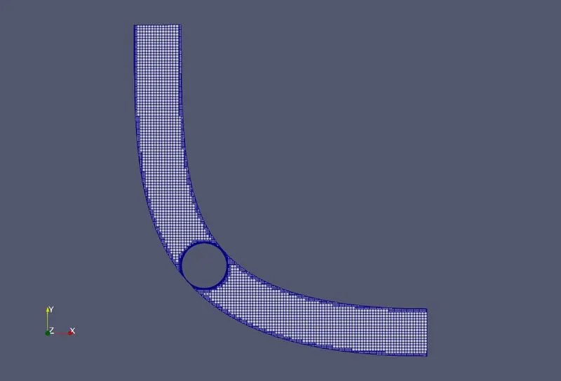
• The mesh size or grid size is 0.001 and in addition to this Fixed embedding is included.
• The fixed embedding is a permanent type and this will include the more number of cell or volumes at the desired location in fixed embedding.

      

      

• Accept the default values given by the post-processing variables.
• Change the output variable values to have more output files.

 MESH:

        

RESULTS:

• The simulation is calculated for 15000 cycles using the Cygwin command prompt.
• Next, the post files are converted to Paraview binary format.

CONTOURS:

• PRESSURE CONTOUR:

         

         

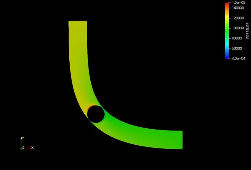
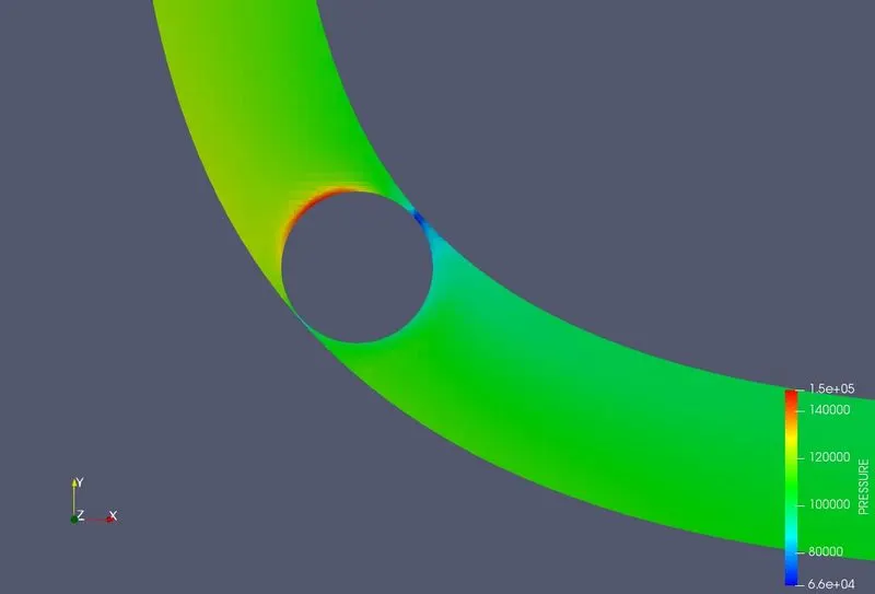
• The above pictures represent the pressure contours. To know the fluid behavior near the throttle wall I have cropped the picture and posted it above. 

• VELOCITY CONTOUR:

       

       

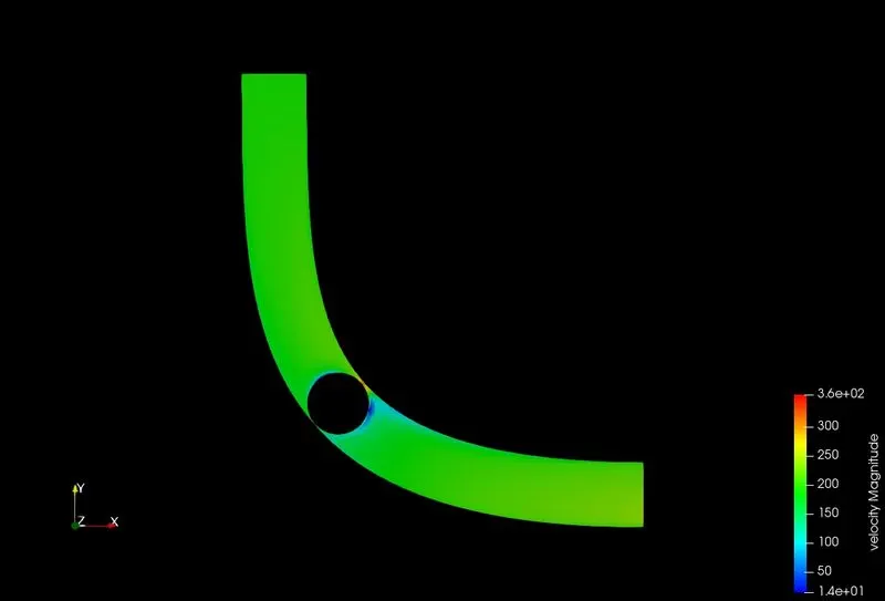
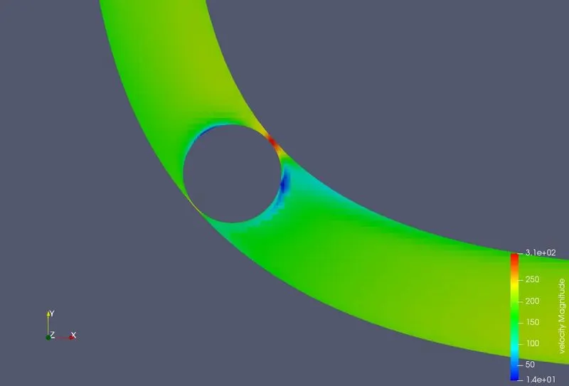
• The above pictures represent the velocity gradients through the pipe and near the throttle valve.

• MASS FLOW RATE:

       

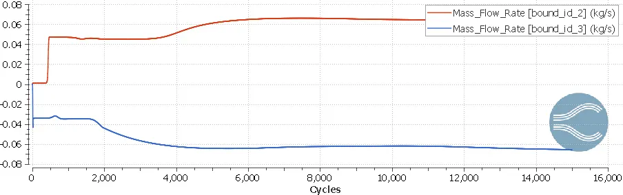
• The above plots depict the mass flow rate of the fluid. The red line represents flow through the outlet and the blue line represents flow through the inlet. 

• TOTAL CELL COUNT:

        

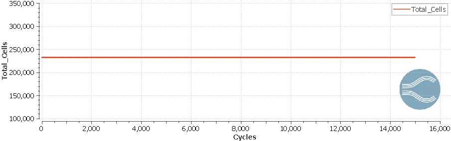
• The total cell count is approximately 240000/-.

• PRESSURE PLOT:

        

     

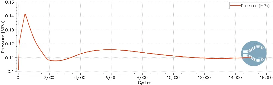
• AVERAGE VELOCITY PLOT:

      

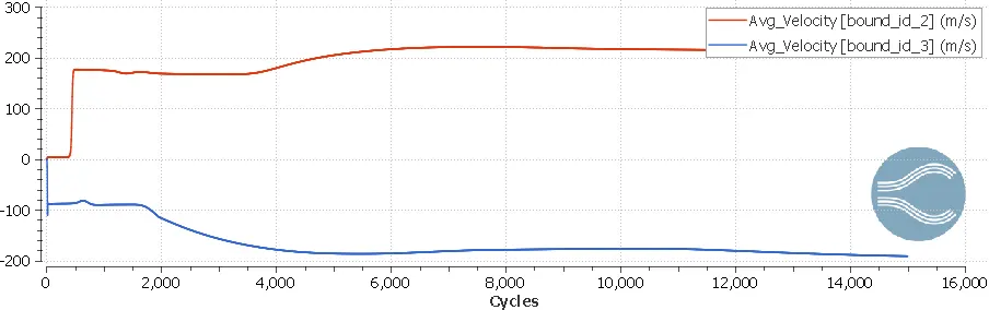
• The above plots depict the average velocity of the fluid. The red line represents flow through the outlet and the blue line represents flow through the inlet. 

 PRESSURE ANIMATION:

 

VELOCITY ANIMATION:

STREAMLINE ANIMATION:

•  CONCLUSION:

1. I would like to declare few points before discussing the results. Firstly, the mesh size is 0.001 and secondly, I have introduced the fixed embedding around the throttle valve as well as at the elbow.
2. This will eventually consume more time. But, the positive outcomes of this are more accurate results, flow pattern, pressure gradients, and velocity gradients.
3. I would like to conclude that, from the above pressure contour the behavior is as predicted it has maximum pressure is at the top and minimum pressure at the bottom of the valve. This is because the flow is interrupted with the throttle valve and the pressure increases on the surface of the valve as shown.
4. The velocity contour is vice-versa to pressure contour. Here, the velocity gradient on the top and bottom valve are minimal i.e. is closer to zero but not exactly zero. The right side of the valve has higher velocity this is due to the sudden decrease in the area in other words decrease in volume.