Week 6: Conjugate Heat Transfer Simulation

Aim: The aim of this project is to simulate the conjugate heat transfer in a pipe.

Introduction: In this simulation, the air is passed through an aluminum pipe, which is receiving a constant heat flux of 10,000 W/m^2 at the outside wall. The object is to understand the phenomena and run the grid dependence test and analyze the effect of the supercycle stage interval in the problem.

Theory:

Geometry Setup:

• The pipe has an inner radius of 15 mm and 5 mm thickness and the length of the pipe is 200 mm.
• The material flowing inside is atmospheric air (77%N2 and 23% O2) In Z direction.

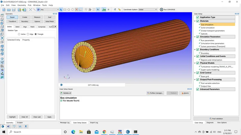
Materials:

Gas Simulation:

• For gas simulation and global transport parameters accept the default values.

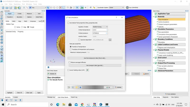
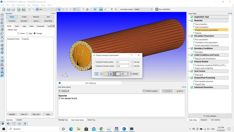
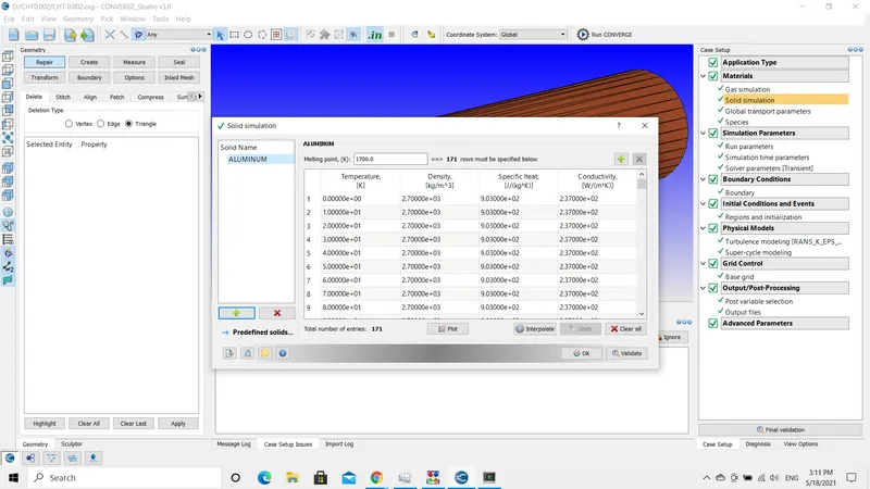
• In this simulation, the material used is aluminum and it is important to enabling the solid simulation to add the material properties.
• In this case, converge has the material properties. In some simulations, we have to manually import the mechanical and thermal properties of the material.

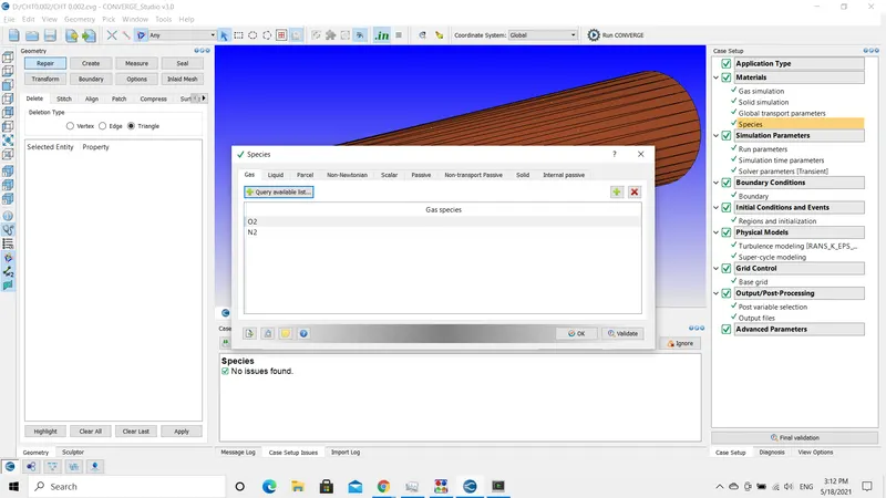
• Include the species inside the tube.
• Oxygen and Nitrogen are the species flowing inside the pipe.

Simulation Parameters:

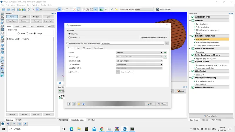
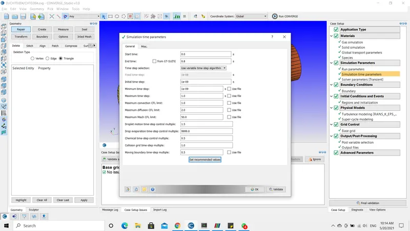
• I am running a transient simulation with a full-hydro solver.

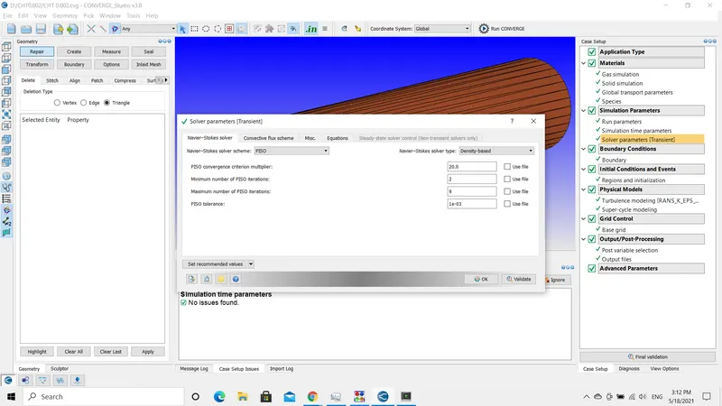
• Solver Parameters: I am using a density-based Navier-Stokes solver.

Boundary Conditions:

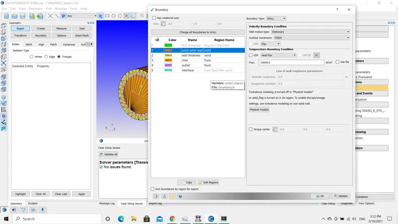
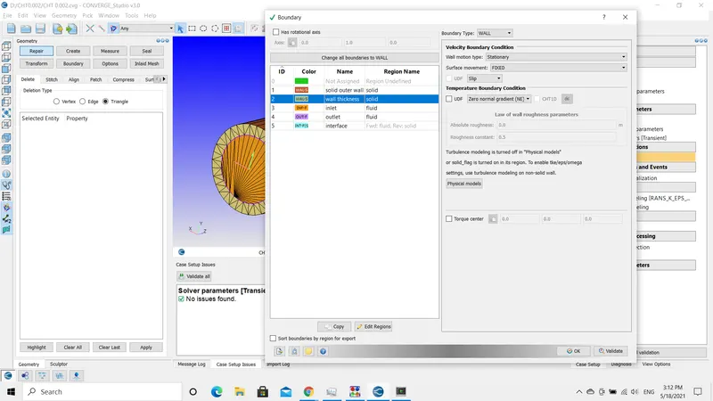
• Both the outer solid and solid thickness have should be assigned slip condition as there is no fluid flowing.
• As this is a CHT simulation the temperature is set to heat flux and 10000 W/m^2 energy is flowing.
• The negative sign indicates that the energy flowing toward the hallow region.

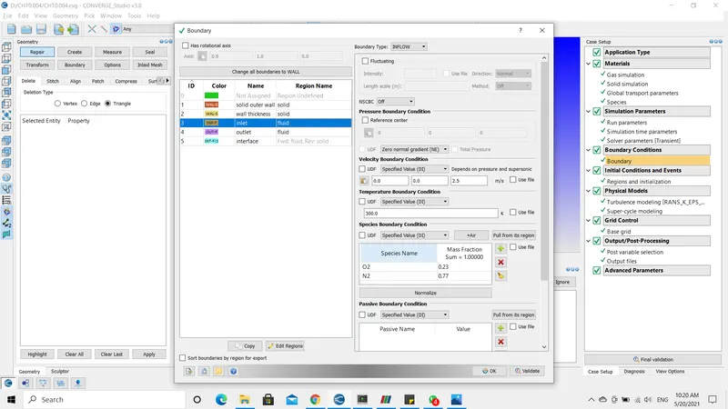
• After calculating the Reynolds number with the above-given value the Velocity is 2.5 m/s.
• I have explained the calculations process in the conclusion part.

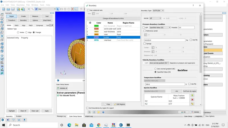
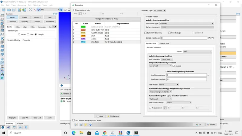
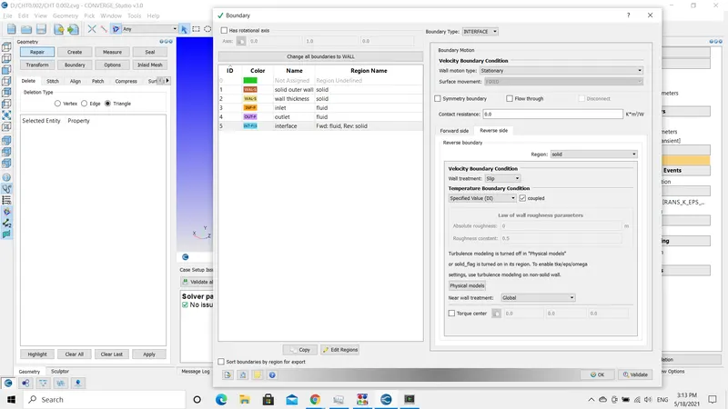
• Interface boundary condition, the surface that is shared by both fluid region and solid region is known as the interface.
• In simulations like conjugate heat transfer, it is important to flag interface boundary conditions to converge the simulation.
• The interface condition has two options forward side and reverse side.
• The forward side is pointed towards the fluid region and the reverse side is pointed towards the solid region.

Initialization Conditions:

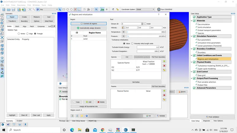
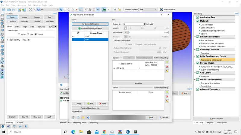
• In regions and initialization, I have introduced two regions for solid and fluid.
• For fluid, the pressure is 101325 Pa.
• For solid, the region ID must be changed to 1 and add the material being used for the simulation as shown in the second picture.

Physical Models:

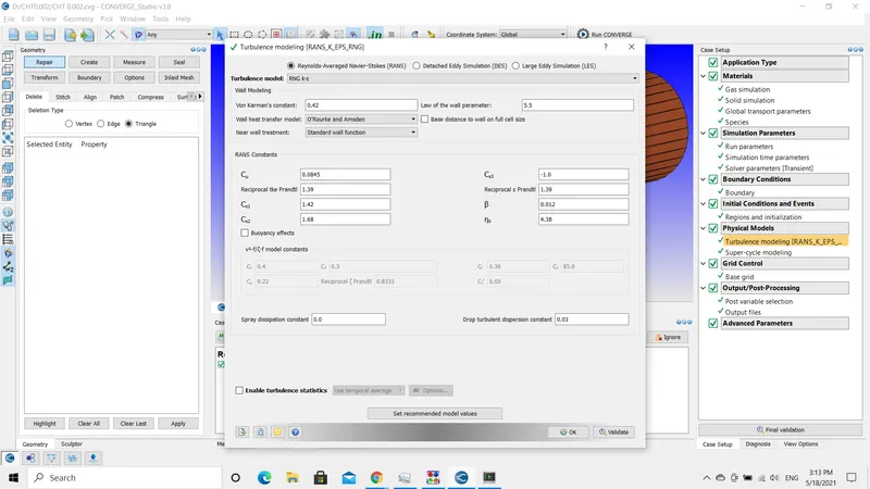
• I have used the RNG K-epsilon methods for the turbulence model.

Super Cycling:

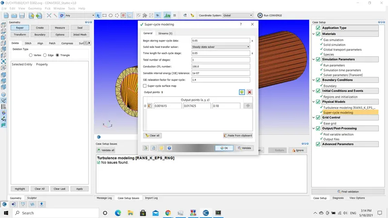
• Super-Cycling is used to obtain the accurate final temperature distribution on the fluid side or solid side.
• In this simulation, I am using it inside the solid thickness and I have also mentioned the location.

Post Processing:

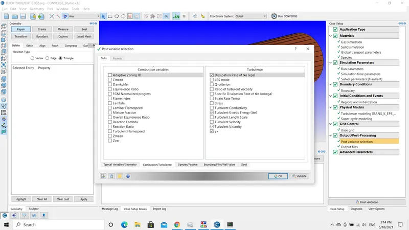
• To find the temperature near the surface of the wall. I have enabled the Y+ in the turbulence model of Post variable selections.
• Converge automatically sets the Y+ value that is suitable for the simulation.

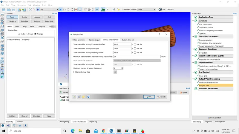
• I am generating an output file at every 0.016 seconds in total I have generated 50 post files.

Results:

• The temperature gradient increases around the wall as it reaches the outlet and this is visible in the below attached animation.

Animations:

• Temperature
• 2mm Grid Size

• 3mm Grid Size

• 4mm Grid Size

• Velocity
• 2mm

• 3mm

• 4mm

• Y+
• 2mm

• 3mm

• 4mm

Plots:

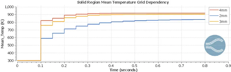
• Mean Temperature Solid Region:

• Mean Temperature Fluid Region:

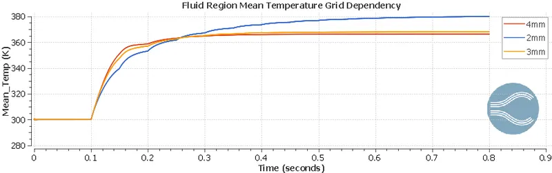
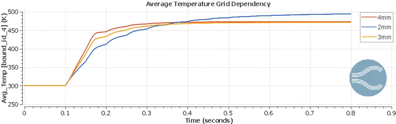
• Average Temperature :

Conclusion:

• Firstly, I would like to conclude that, I have performed the simulation on three different grid sizes i.e., 2mm, 3mm, and 4mm and I have uploaded the results above.
• In this simulation, the Reynolds number is 7000 and the inlet velocity is 2.585
• `Re=(rho vD)/mu` = `=> V= (7000*1.81*10^-5)/(1.225*0.04)=2.585`
• Y+ wall function is also enabled. In converge, the software itself calculates the Y+ and applies for the suitable number.
• To apply Y+ go to post processing => turbulence model => check the YPLUS option.
• From the above results, it is visible that the mesh size of 2mm has the best output. It is always preferable to have a smaller grid size in order to capture the gradients with high accuracy.
• And the Y+ generated for the 2mm base grid is also smaller and efficient compared to other grid sizes.
• From the animation, we can understand that the fluid flows along the Z direction. As the fluid moves towards the outlet the fluid temperature gradient increases because the solid thickness is generating or emitting 10000 Wm^2 energy into the pipe.
• This temperature variation is accurately captured in the 2mm grid size animation.
• The plots also depict the same information as in the animations. In all the plots that show the temperature value, the grid size of 2mm shows the higher temperature.
• We can use the super cycle method in multiple locations. In this simulation, I have used it in only one location.
• In the end, It is proven that the lower the mesh size greater the accuracy.