Week 10: Project 1 - FULL HYDRO case set up (PFI)

AIM: To perform a Full-Hydro simulation of an Internal Combustion Engine of Port Fuel Injection type model.

INTRODUCTION:

• In this project, I will explain the setting required to perform the Full-hydro simulation.
• In the previous paper, I have focused on setting up the No-Hydro simulation and generating the inlet and exhaust port animation.
• This paper contains more information regarding the fuel parcels, setting up nozzle location, combustion modeling, the importance of chemical kinetics, AMR, Fixed Embedding.

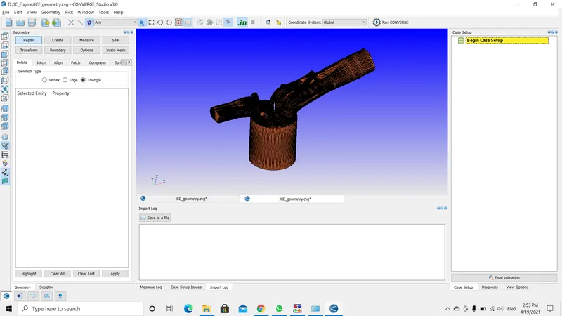
THEORY: I begin with the starting process. Initially import the geometry into the convergent software and start the case setup using crank angle-based IC_Engine.

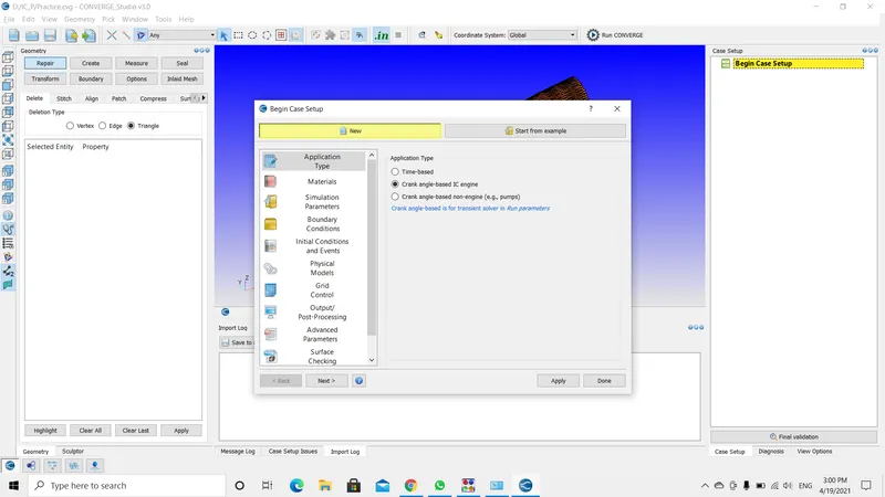
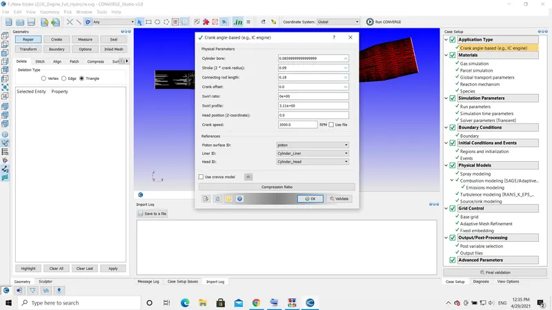
• The above picture shows the crank angle-based IC_Engine setup. The values for this setup are provided in the challenge section.
• In the reference field initially, the ID's are not available we should flag the boundaries and name them in order to get the paths in the reference section.
• I have flagged the boundaries prior to setting up or feeding the values into the application dialogue box.

MATERIALS:

There are a couple of options to be enabled in this section.

1. Parcel Simulation.
2. Reaction Mechanism.
3. Species.

After enabling the above parameters, start setting up the section.

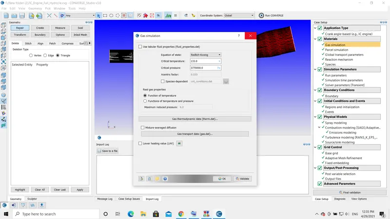
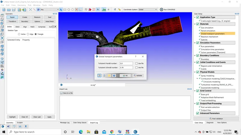
GAS SIMULATION and GLOBAL TRANSPORT PARAMETERS: Use the default options for this parameter. However, we will be using atmospheric air with fuel.

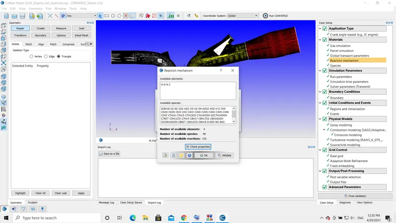
REACTION MECHANISM: It is always advisable to set up a reaction mechanism before setting up the parcel simulation. As we may not find the option we should enable.

• In the reaction mechanism, upload the mech.dat file and check properties. Initial this will show some error because the mechanical files that contain the species in the mech.dat are incomplete without thermodynamic properties.
• So, there will be another file called therm.dat. We can upload the input file by File-> Import -> Import Input File(s) and here upload the desired file.
• Now check the properties, This time the reaction mechanism shows zero errors.

PARCEL SIMULATION:

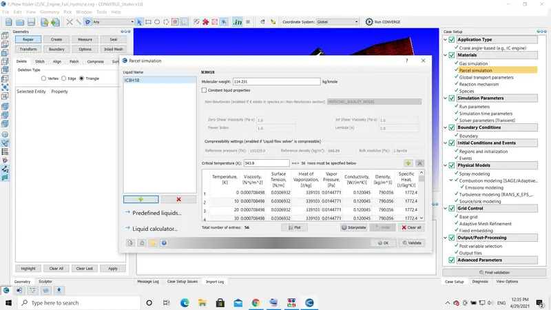
• To set up the parcel simulation, add a new parcel by using the ADD button at the bottom of the dialogue box and enter IC8H18.
• Before completing the species name there will be a suggestion pop up, after selecting the option the properties of the species will appear in the dialogue box.

SPECIES:

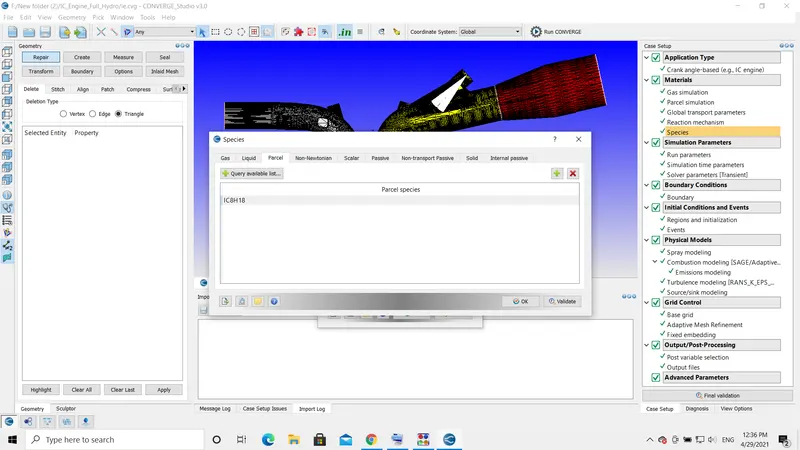
• In species, enable the parcel option and add the IC8H18 species as shown in the below picture.
• To introduce a new species click on the "PLUS" button on the right side and enter the title.
• With this, the Material setup is completed.

SIMULATION PARAMETERS :

RUN PARAMETERS :

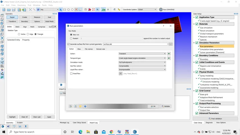
• In run parameters, I am using a transient-based solver with Full-Hydrodynamic mode.

SIMULATION TIME PARAMETERS :

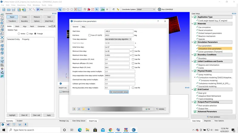
• The starting and ending time is -520 degrees and 120 degrees respectively.
• For other values, I have followed the information provided on the challenge page.

SOLVER PARAMETERS :

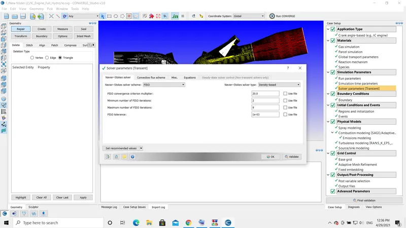
• In solver, parameters use the density-based Navier-Stokes solver.

Boundary Flagging:

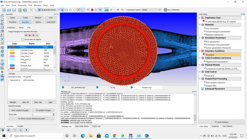
• Boundaries in this type of geometries are complex to flag. I have also used boundary fencing to divide certain regions.
• initially, when I diagnosed the setup I found many errors, and those errors are solved one by one after flagging the boundaries.

First flag the piston. ie., the bottom surface.

• Next, the cylinder liner.

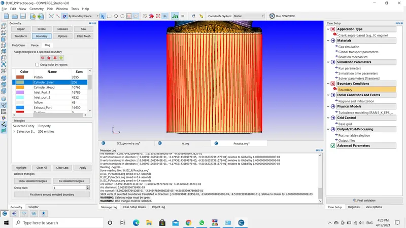
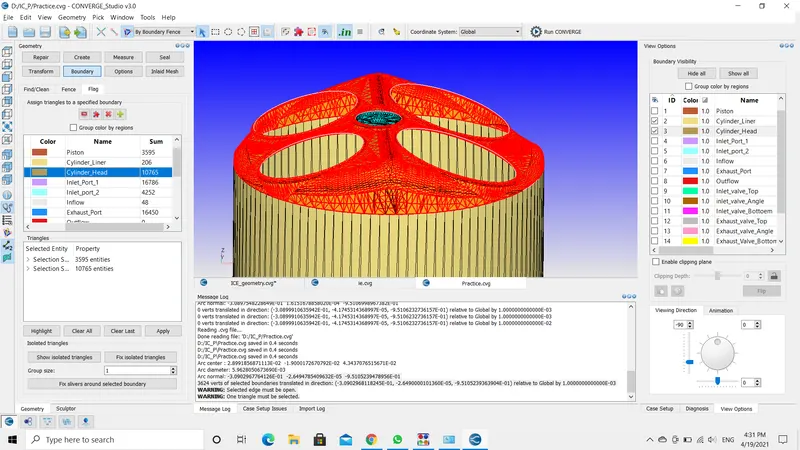
• Next, cylinder head. There is some difficulty in flagging the cylinder as the inlet valves are intersecting the inlet port. This problem has been resolved by translating or moving the valves a little bit.

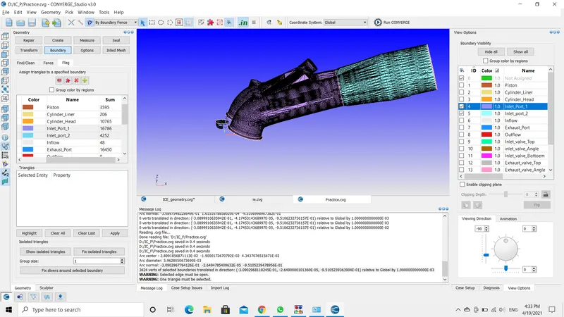
• Next, the intake port. Here the intake port has been divided into two parts intake port 1 and intake port 2. This division has been done using the boundary fencing option.

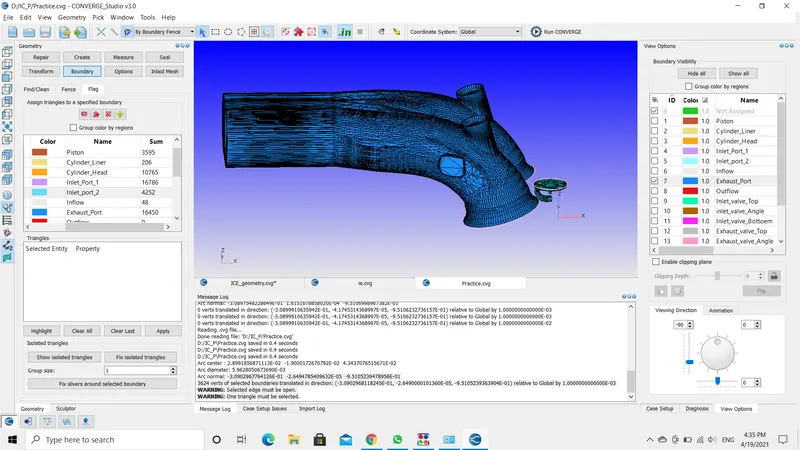
• Now the exhaust port. The exhaust port is not divided as the intake port.

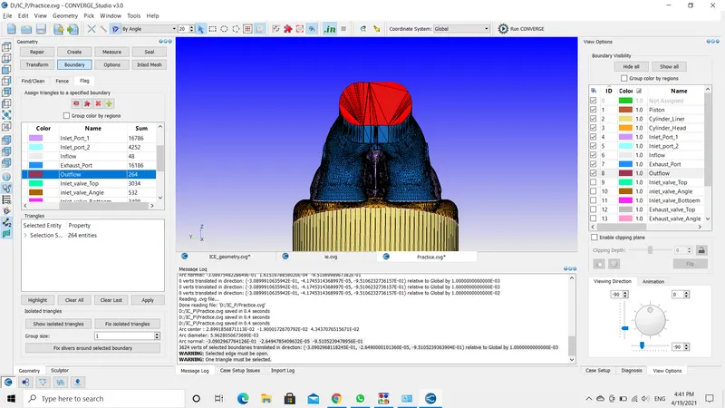
The inflow and outflow boundaries

INFLOW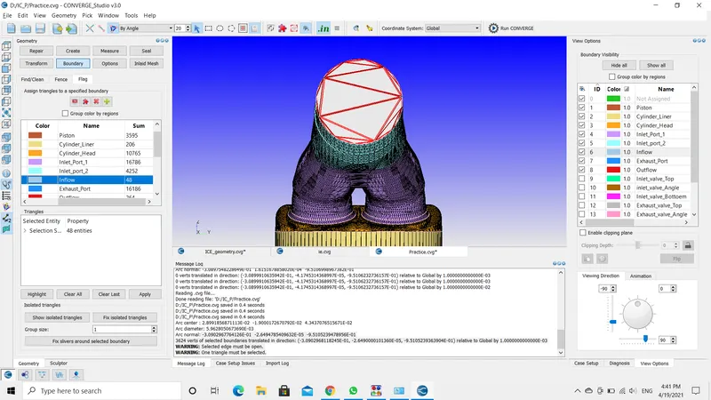

OUTFLOW

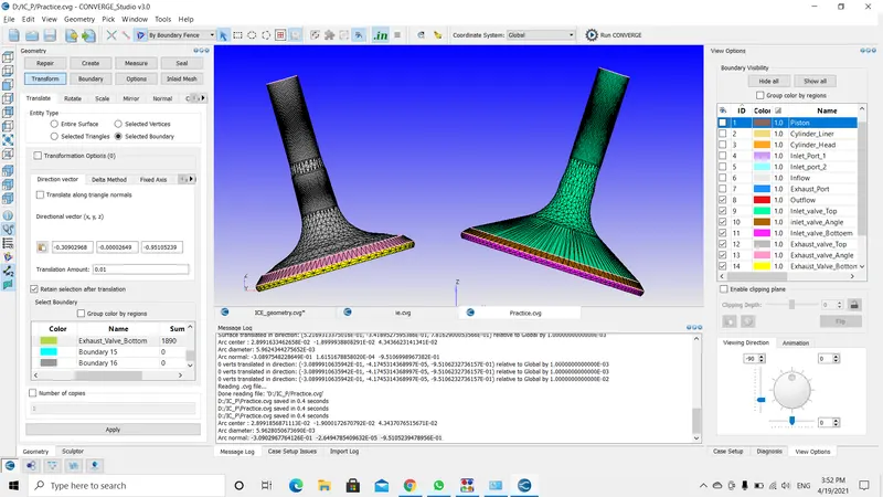
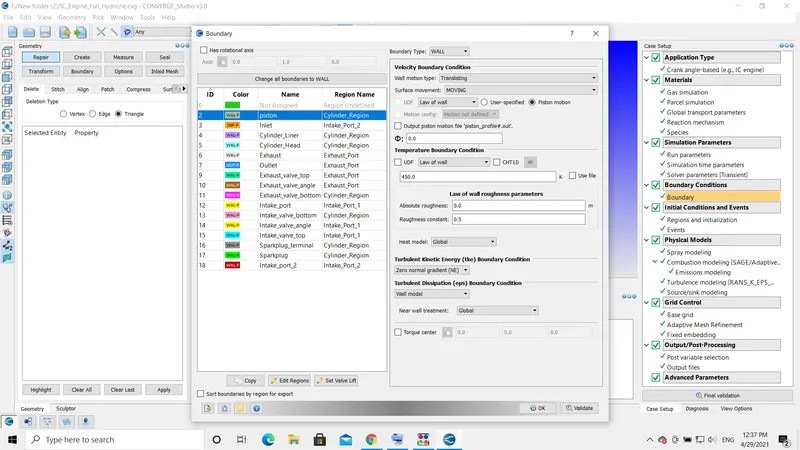
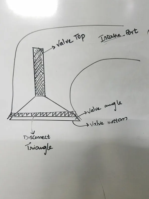
• Coming to inlet and exhaust valves. These valves are divided into three parts namely valve top, valve angle, and valve bottom as shown below.

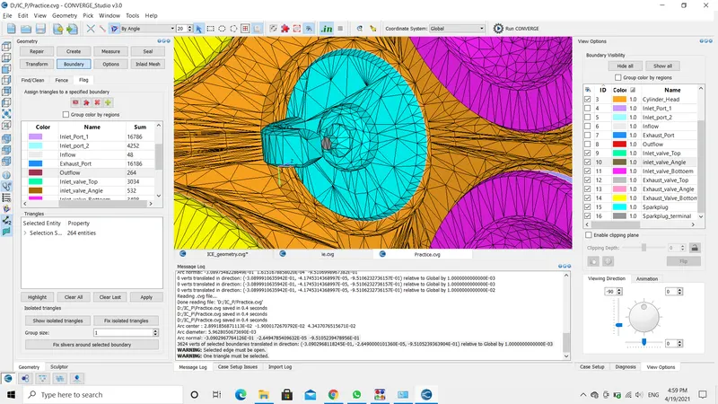
• Lastly the sparkplug. The sparkplug tip separately flagged and the sparkplug terminal. This is because due to the temperature difference. The tip has a greater temperature.

• With this, I have completed flagging the boundaries.

• Boundary conditions parameters are also provided on the challenge page, It is important to follow those values to get the correct output.

Initialize Conditions and Events:

• In section, I have enabled four new regions namely Cylinder_Region, Intake_port_1, Intake_port_2, exhaust_port.
• This is done because, in an engine the temperature, pressure, and chemical characteristics not the same in all locations. So, to describe the characteristics and mass fractions four different regions are introduced.

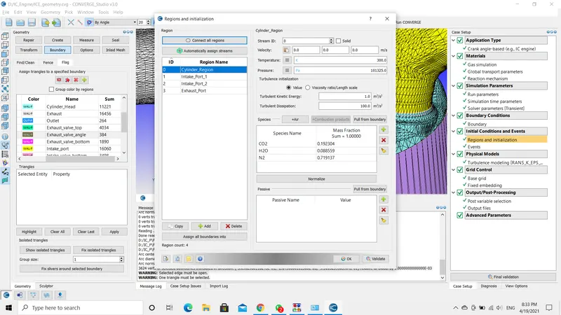
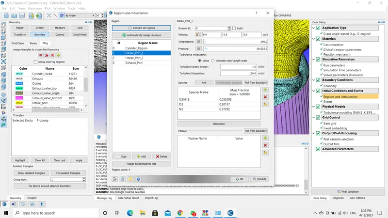
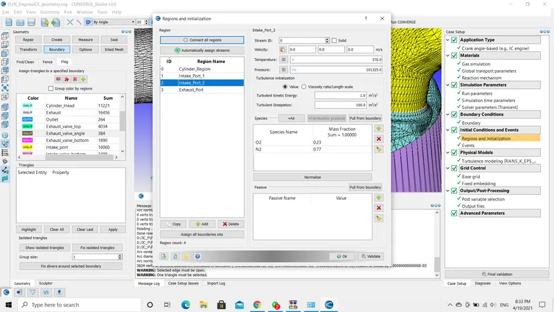
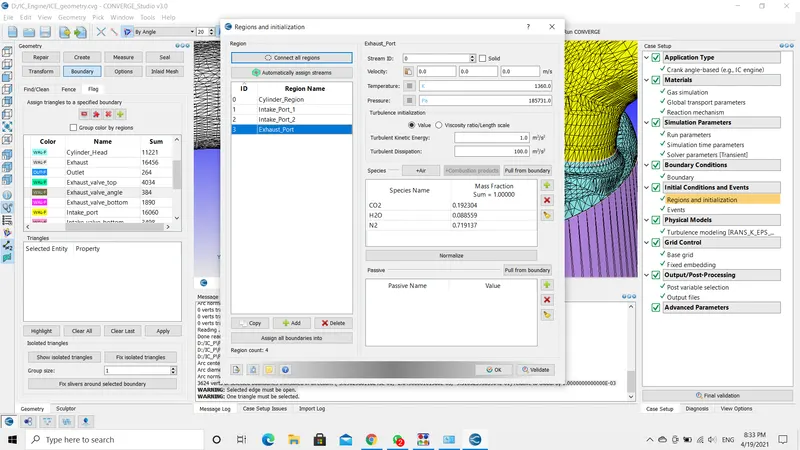
• The above pictures display the mass fractions of each species that are involved in the simulation.

EVENTS:

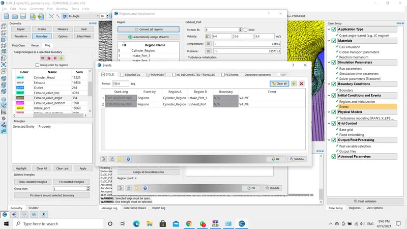
• Events are used to allow the fluid flow(air-fuel mixture) between two boundaries or regions. The flow can be done in sequential order or in permanent type.
• In this, I have enabled two types of events sequential and permanent.
• In sequential type, it allows the fluid flow in the specified period and restricts the flow in other time intervals.
• To determine the time intervals, I have opted for Valve settings to the Event section. This automatically sets the time intervals of valve opening and closing.

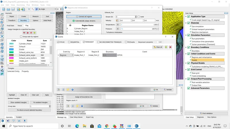
• On the other hand, as I have divided the intake port into two boundaries intake port 1 and intake port 2. I have implemented a permanent opening event between these two boundaries.

PHYSICAL MODELS :

TURBULENCE MODELING :

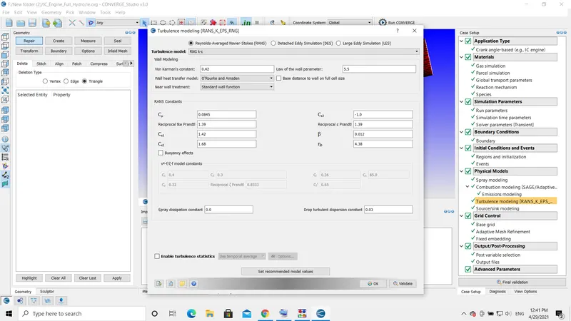
• For turbulence modeling, I have used the RNG K-Epsilon method with below mentioned values.

SPRAY MODELING :

• It is the most arduous task to set up the spray modeling.
• The spray modeling has several fields to be filled.
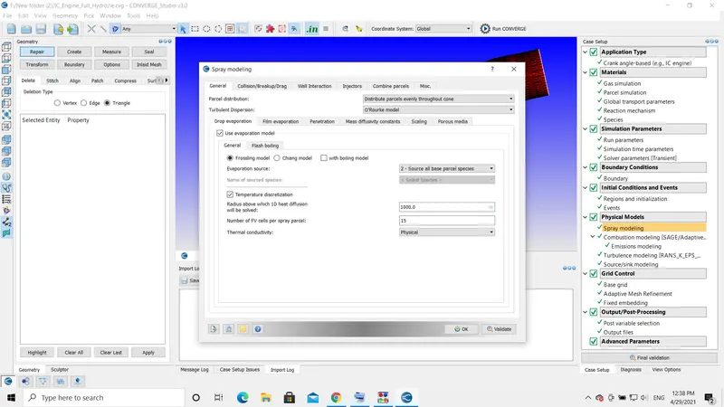
• In General setup, the parcel distribution is set to Distribute parcels evenly throughout cone.
• Turbulent dispersion is set to the O'Rourke model.
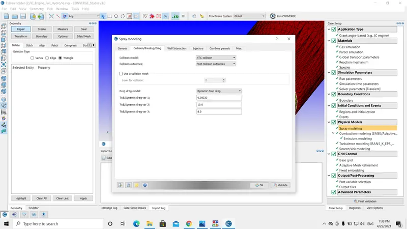
• Collison model to NTC collision.
• Collision outcomes to Post-collision outcomes.

SPRAY MODELING(INJECTORS):

• In this simulation, the nozzle position is outside the cylinder head i.e., in the intake_port_2 boundary as shown in the picture.
• This injector has four nozzles, and each nozzle flow direction is at different angles as shown.
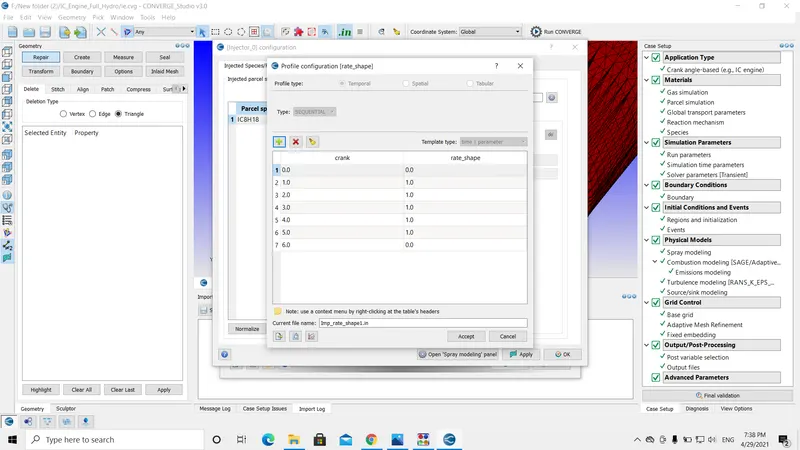
• While setting the injector set up first, include the parcel species. In this simulation, the species is IC8H18 with a mass fraction of 1.0 and configure the profile graph to seven parts.
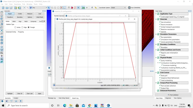
• Finally, the output of the profile plot represents a conical shape.

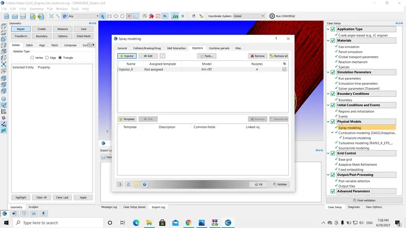
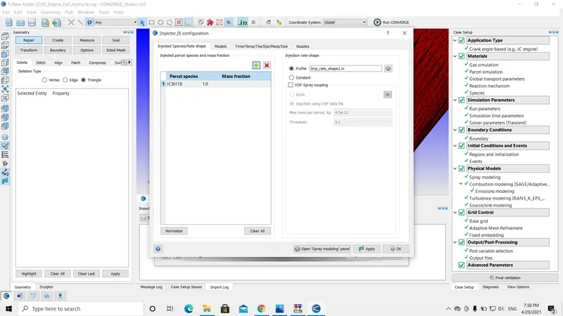
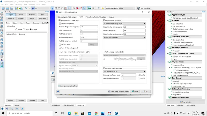
• The injector model used is the Kelvin-Helmholtz model. To set up the values for the field we can use recommended values option on the bottom left side of the dialogue box.

• It is important to determine the start of injection, duration of injection, and total mass of injection. These values are also provided on the challenge page.

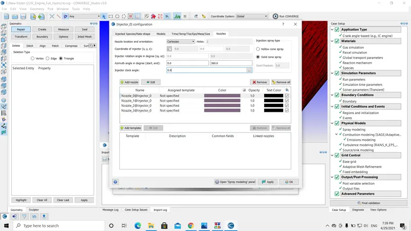
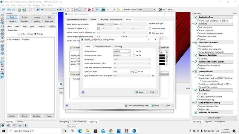
• Finally, as mentioned in the above line regarding the four nozzle injections, introduce four nozzles by selecting the add nozzle button and use the values for each nozzle flow direction or nozzle angle that are provided on the page.

COMBUSTION MODELING:

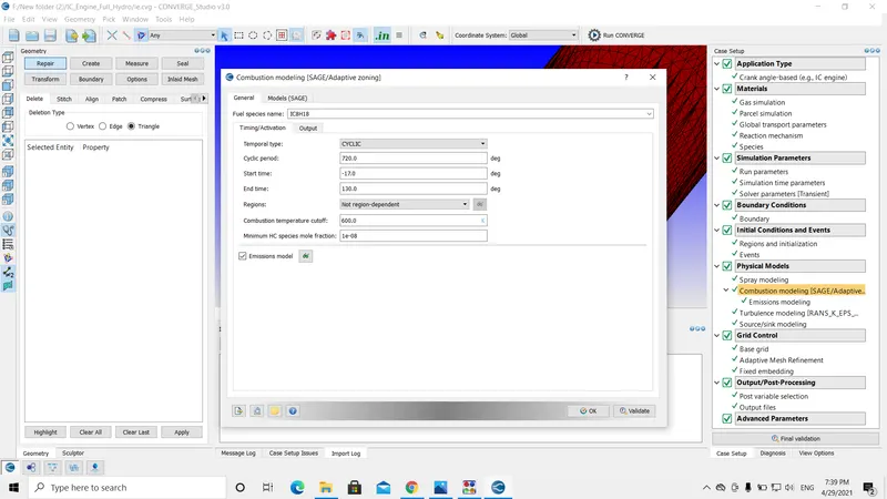
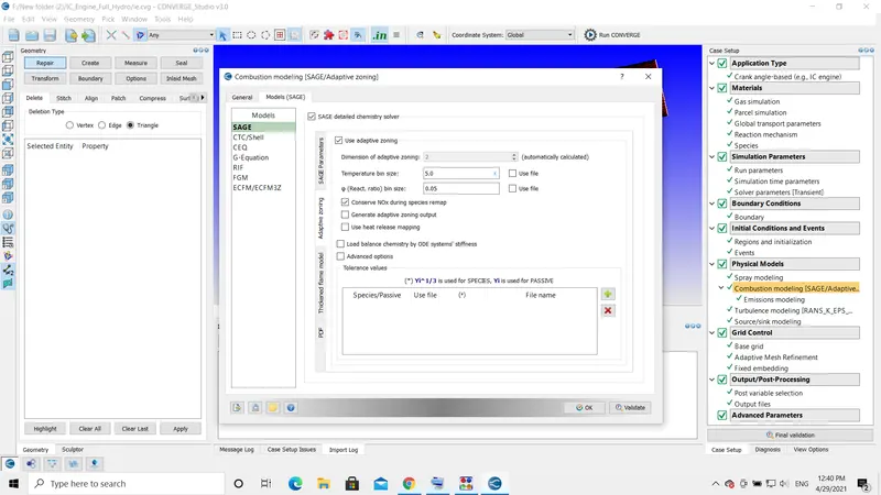
• In this combustion modeling, I have used the SAGE model by using the values provided on the challenge page.

SOURCE/SINK MODELING:

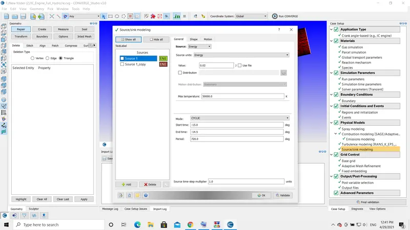
• In this section, I am determining the amount of energy emitted by the spark plug.
• I have configured two energy sources at different time intervals at the same location.

GRID CONTROL:

BASE GRID:

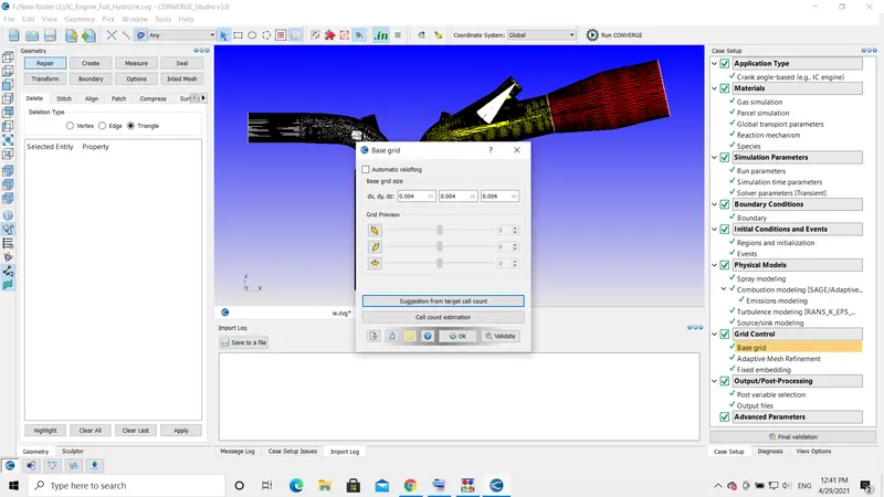
• The rough cell count is estimated to be 15007 cells.

ADAPTIVE MESH REFINEMENT :

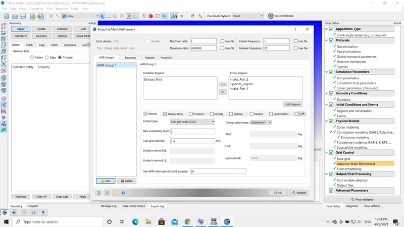
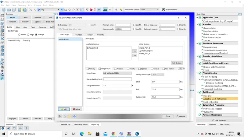
• I have used AMR for temperature and velocity in intake ports 1 & 2, and cylinder head.
• And the timing used is cyclic type, between -17 and 135 degrees.

FIXED EMBEDDING :

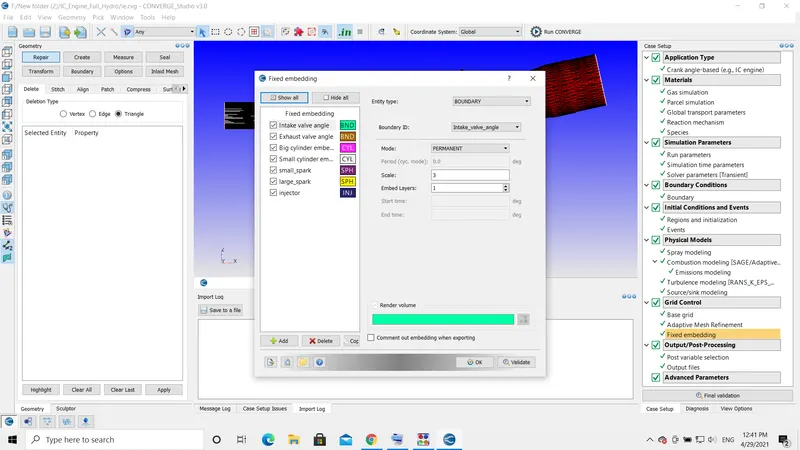
• I have implemented the fixed embeddings in the intake valve angle, exhaust valve angle, cylinder head, cylinder liner, nozzle, sparkplug, and injector.

OUTPUT/POST-PROCESSING:

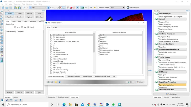
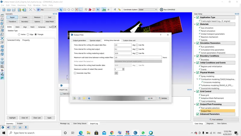
• The values provided in the post variables and output files by default are correct and we can proceed using these values.

EXPLAINATION:

• In this section, I will illustrate the apprehension behind selecting above mentioned values and models.

• Firstly, I will demonstrate RING TRIANGLES.
• In the simulation, the valves do not close completely there will be a small gap or minimum lift as shown in the below picture. If these valves are closed or moved backward there might be an intersection error.
• Every valve in this simulation is divided into three boundaries Valve top, angle, and bottom. These boundaries are assigned to different regions. The Valve angle and valve top are assigned to intake_port and the valve bottom is assigned to the cylinder region.
• This helps in identifying the location of the parts and also the temperature and pressure inside the cylinder and intake port are not the same. Multiple regions are created to describe the maximum pressure, temperature, and chemical kinetics involved in it.
• On the other hand, to restrict the flow through these small gaps CONVERGE creates a DISCONNECT TRIANGLE to prevent the air-fuel mixture from entering the combustion chamber with the help of the regions and boundaries.
• The flow cannot enter into the cylinder when these triangles are present or active and the flow can pass through in the absence of these triangles.
• The disconnect triangles are operated using EVENTS.

NOZZLES & SPRAY MODELING:

• Fuel after entering into the combustion chamber is affected due to the turbulence characteristics. O'Rourke model gives better performance in solving the turbulence modeling.
• Collision: To calculate the collisions in the Lagrangian spray simulation NTC model is used. In general, when the fuel enters the droplets per parcel is not the same all the time the number varies. So, the NTC (no time counter) is several orders of magnitude faster and slightly more accurate than methods.
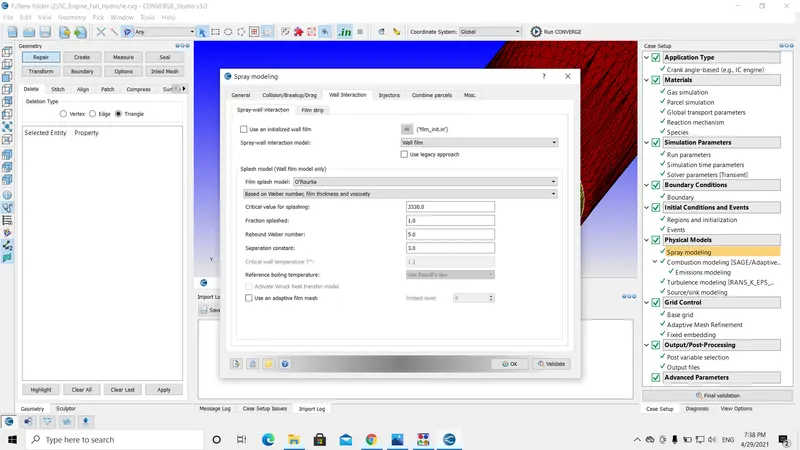
• Wall Interaction: I have enabled the spray wall interaction model to wall film, this helps in reflecting or splashing the droplet when it hits the wall. The film model is set to the O'Rourke method.
• Injector: In the injector, I have included the fuel that I am using for the simulation i.e, isooctane (IC8H18).
• I have also provided a profile for rate shape to a trapezoid. Converge utilizes this profile to inject the total mass according to the given time that I have provided.
• Kelvin-Helmholtz and Rayleigh-Tailor models are the industrial standard models for fuel injection with standard values. These values describe the parcel breakup and time taken for a parcel to get unstable.
• Nozzles: As I am solving a port-fuel injection simulation, the nozzles are positioned before the intake valves as shown in the below picture. I have positioned four nozzles by using the cartesian method. The nozzle centers and align vectors values are provided on the challenge page.
• On the other hand, we can also locate the center by using the measure option.
• The final part of the nozzles is the injection pressure. The injection pressure is automatically solved by the converge by using the initial conditions such as rpm, injection duration, total mass injected, discharge coefficient.

COMBUSTION MODELING:

• SAGE type of combustion model is used and multi-zone model to speed up the combustion calculations.
• Firstly, the type of fuel used for combustion is mentioned, Next the start time, end time, and the cyclic period.
• For the start time, the combustion model is set to start a few degrees before the spark takes place so as to initiate the combustion calculation.
• The end time is the same as the exhaust valve closing time.

SOURCE/SINK:

• An energy source is required to begin the combustion, the source term is responsible for temperature change, the temperature affects the chemical kinetics and thus causes the byproducts.
• I have enabled two source models in a spherical shape. The location of the source is at the sparkplug center, the location is also provided on the challenge page.
• The source is cyclic, with 720 cyclic periods.
• The energy emitted by the first source is 40 millijoules and the energy emitted between -15 degrees and -14.5 degrees.
• In the second source, the energy emitted is 20 millijoules, and the energy emitted between -15 degrees and -5 degrees.
• It requires more energy to break down the fuel so we use 20 MJ for 0.5 degrees in the first source and to continue the conduction process we use the second source with 20 MJ of energy for 10 degrees. For the first 0.5 degrees of the cyclic period, I have provided 40 MJ of energy at the same location to break down the fuel parcels evenly.

ADAPTIVE MESH REFINEMENT (AMR):

• In numerical analysis, AMR is a method of adapting the accuracy of a solution within certain sensitive turbulent regions of simulation, dynamically and during the time the solution is being calculated.
• When solutions are calculated numerically, they are often limited to pre-determined quantified grids as in the cartesian plane which constitutes the computational grid, or mesh.
• Many problems in numerical analysis, however, do not need a uniform precision in the numerical grids used for plotting or computational simulation and would be better suited if specific areas of graphs need precision. AMR provides such a dynamic programming environment for adapting the precision of the numerical computational based on the requirements of a computation problem in specified loactions.
• Subgrid criteria (SGS) is an integral part of AMR. As the AMR is used for different parameters Temperature, Velocity, Pressure, and Species, etc.
• The SGS is provided with a predefined value. If the parameter exceeds the specified value in the SGS, the AMR automatically enables.

FIXED EMBEDDING:

• Fixed Embedding is a smart feature. It helps in adding extra mesh in specified locations.
• This offers numerous benefits including the ability to apply more cells near a wall and get an increase in accuracy, and running a fast coarse mesh without distorting the geometric representation.
• The following regions and boundaries included in fixed embedding including, Intake valves, Exhaust valves, Cylinder region, nozzles, and sparkplug.
• The fixed embedding act as an additional refinement in that areas.
• For example in the cylinder region, the energy emitted through the source term resides for a longer period of time and numerical diffusion takes place.
• The fixed embedding is active for a very small duration of time, helps in capturing the better seed values, temperature gradients.
• This also initiates AMR to be activated in that region or a particular area.

What is the compression ratio of this engine?

The compression ratio (CR) is defined as the ratio of the volume of the cylinder and its headspace (including the pre-combustion chamber, if present) when the piston is at the bottom of its stroke to the volume of the headspace when the piston is at the top of its travel (‘top dead center’, TDC). Typically, petrol engines have a CR of 8–10, while diesel engines have a CR of 15–20. The CR of petrol engines is limited by the requirement that the fuel burns uniformly in the cylinder and does not ignite thermally prior to the spark (so-called ‘engine knocking’). In a spark-ignition engine, the CR at which pre-ignition takes place is determined by the octane number of the petrol. High-octane fuel permits a high CR. Until about 30 years ago, lead tetraethyl was added to petrol as an anti-knock agent. This was phased out for environmental reasons and non-toxic additives are now sometimes used. Improvements in engine design over recent years have, however, led to satisfactory compression ratios with lower octane fuel.

Effects:

The compression ratio, in this case for a realistic engine it is the effective one, has two effects on combustion. The first, and obvious effect, is on the thermodynamic cycle. The pressure and temperature at the end of compression will be affected by the compression ratio, with a higher compression ratio increasing both these parameters. Compression ratio will also have a significant effect on the geometry of the combustion chamber, and a higher compression ratio will often result in a combustion chamber of a narrower aspect ratio. This means that the flame will contact the piston earlier and this will tend to reduce the rate of heat release. The compression ratio of the base engine was both increased and decreased.

`CR= (V_d+V_c)/V_c`

`CR`= static compression ratio

`V_d`= displacement volume

`V_c`= clearance volume

Where

`V_t = V_d+V_c`

`V_t`= sroke volume

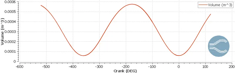
`V_t and V_c` can be derived through the below plots

`V_t =`0.000574219

`V_c =`0.0000575439

`CR = V_t/V_c` = 10.

Compression Ratio = 10.

Why do we need a wall heat transfer model? Why can't we predict the wall temperature from the CFD simulation?

• It is necessary to know the heat loss through the walls of an engine during the optimization, as it influences power, efficiency, emissions, and engine components of thermo-mechanical reliability. Because of the difficulties involved in the heat transfer mechanism, it is complicated to predict. Another significant aspect of the optimization procedure of these engine technologies is the study of heat transfer through the walls of the engine and this has a direct impact on the power & efficiency of the engine as more heat is being lost as less power is transferred to the crankshaft. On the other hand, this also affects the thermal energy passing through the exhaust port, for which different after-treatment tools are required to analyze. The gas temperature with oxygen concentration is key to the formation of Nitrogen oxide which affects the hydrocarbons and Soot.

• Why we cannot predict the wall temperature from CFD simulation: For instance, let us consider an air-cooled IC_Engine. In this type of engine, the engine temperature is reduced by air passing through the fins and this is also called natural convection. To calculate the wall temperature or wall heat transfer in CFD, we should set up a computational mesh that includes the surrounding environment and this analysis or simulation will be costly and a lot of calculations are involved in this. To overcome this, CFD software has a "Heat Transfer Co-efficient" value with this we can predict the heat lost through walls. These values are widely available and these values differ for the different velocities of the wind or air. We can use this data and provide it as input.

Combustion Efficiency:

• In general, The exhaust gas of an internal combustion engine contains unburnt particles such as CO, H2, hydrocarbons, soot.
• Under lean operation conditions, the number of incomplete combustion products is small. Under high fuel operating conditions, the volume increases due to the supply of incomplete oxygen into the combustion chamber. If a fraction of the fuel's chemical energy is not fully released inside the engine during the combustion process, it is useful to define combustion efficiency.
• Combustion efficiency is defined as `n_c=(H_r(T_a)-H_p(T_a))/(m_f*Q_(hv))`

`H_r`= enthalpy of the reactant (internal energy) [J]

`H_p`= enthalpy of the product (internal energy) [J]

`T_a`= ambient temperature [K]

`m_f`= mass of the fuel used per cycle [kg]

in other words

`n_c=(output power)/(Input power) * 100`

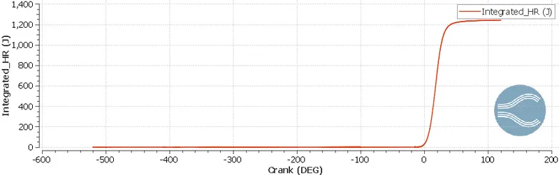
Output Power=`H_r(T_a)-H_p(T_a)`

we get the output power value from the below plot =1241.16 J

Input power = 444000*3e-5

`n_c` =1241.16/(44*10^6*3e-5) * 100

=1241.16/1320*100

=0.94027*100 = 94.027%

Finding power and torque of engine by using engine performance calculator :

1

2

3

4

5

6

7

8

9

10

11

12

13

14

15

Cycle (number)

CAD_from (deg)

CAD_to (deg)

Duration (deg)

Gross_Work (N*m)

IMEP_(Gross) (Pa)

CAD10 (deg)

CAD50 (deg)

CAD90 (deg)

PFP (MPa)

PFP_CAD (deg)

HRR_Peak (J/deg)

HRR_Peak_CAD (deg)

Net_Work (N*m)

PMEP (Pa)

1.000000e+00

-1.200900e+02

1.201100e+02

2.401990e+02

4.686460e+02

8.964280e+05

6.837170e+00

1.846230e+01

3.170100e+01

3.888840e+00

2.397000e+01

5.935620e+01

1.884470e+01

0.000000e+00

-1.000000e+00

Power(P) = (`2*pi*N*T`)/60

Power = Work/Time.

Work = 468.64 N-m

Time = Duration(deg)/Degrees Per Second =240.199/18000=0.0133 Seconds.

Power = 468.64/0.0133 = 34819.12914 KJ or 34.819 KW

N (RPM) = 3000

P=(`2*pi*N*T`)

34.819*60/2*pi*3000 =T

T= 34819.14*60/2*pi*3000

T= 11083 N-m

What is the significance of ca10, ca50, and ca90: The ca10, ca50, and ca90 depict the crank angle moment at different stages of combustion. In other words, the percentage of fuel burned completely at certain crank angles.

• ca10: It shows that 10% of the fuel is burnt at a 6.837170e+00 crank angle.
• ca50: It shows that 10% of the fuel is burnt at a 1.846230e+01 crank angle.
• ca90: It shows that 10% of the fuel is burnt at a 3.170100e+01 crank angle.

The crank angle values are derived from the engine performance tool from the converge software and other parameters are also tabulated above for reference.

RESULTS :

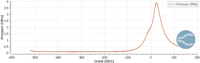
• Pressure Plot

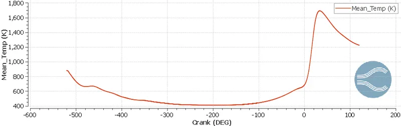
• Temperature Plot

• Volume Plot

• Integrated Heat Release Plot

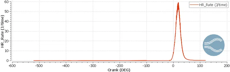
• Heat Relase

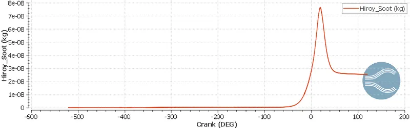
• Soot Plot

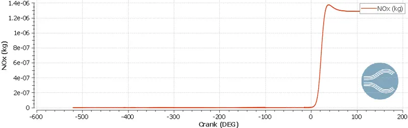
• NOx Plot

Pressure Animation:

Temperature Animation:

Velocity Animation:

CONCLUSION :

• In this simulation, the simulation start time is -520 degrees and the end time is 120 degrees.
• At -520 degrees the exhaust port is opened a little, the animations start with the closing of the exhaust valve and the piston starts moving towards Top Dead Cell.
• Next, as the exhaust valve closes the nozzle starts spraying the fuel, The inlet valve opens, the air-fuel mixture enters the cylinder/combustion chamber, the piston compresses the mixture and spark ignites the mixture thus combustion occurs.
• The pink color represents the fuel parcels entering the combustion chamber. While the nozzle sprays the fuels some droplets fall on the walls and with the help of the O'Rourke film method it the droplets reflect and carried into the cylinder region.
• Inside the cylinder region, the fuel is distributed equally.
• The first animation shows the pressure contours inside the cylinder. Before completing the compression stroke the maximum pressure inside the chamber is 1.2e+05 Pascals and the spark begins at -15 degrees crank angle and lasts for 10 degrees.
• The second animation shows the temperature contour, the peak temperature inside the chamber is 1.2e+03K. The exhaust temperature could be slightly lesser than 1100 K.
• The last animation shows the velocity contour, The fluid travels around 200 m/s through the exhaust port.
• The plots show the Pressure, Temperature, Volume, Heat Release, Integrated Hear Release Rate, Soot, and NOx emissions.
• All the plots possess a peak value between 15 and 20 degrees crank angles. At this point, the piston is near the Top Dead Cell.
• Between this crank angle period, the pressure value is close to 4 MPa, and the temperature is around 1700 K.
• It shows that the Integrated-HR is 1241 joules and HR is a peak at 20 degrees crank angle.
• The Nox emission is less than 1.4e-06 which is less than 2 ppm that under an acceptable level.
• However, we cannot say the engine has higher efficiency and produces fewer pollutants without comparing to other engines.