Week 7: Shock tube simulation project

Aim: The main objective of this analysis is to perform shock tube simulation using the transient solver method and animate the pressure and temperature changes inside the tube.

Introduction: The shock tubes are generally utilized to study chemical kinetics. The geometry consists of a long square tube where both ends are closed. in the middle of the tube, a diaphragm is placed to divide the high-pressure region and low-pressure region. During the simulation when the diaphragm is removed the high-pressure fluid enters into the low-pressure region and thus makes compression and expansion waves.

Examples of this type of simulation are auto-ignition systems. The tube is filled with fuel and air in the two chambers. Due to the shock waves and the increase in temperature, the air-fuel mixture is going to auto-ignite. This simulation shows the time-lapse of the air-fuel mixture to ignite, this data is used to improve the engine and reduce the carbon footprints.

Theory

Geometry:

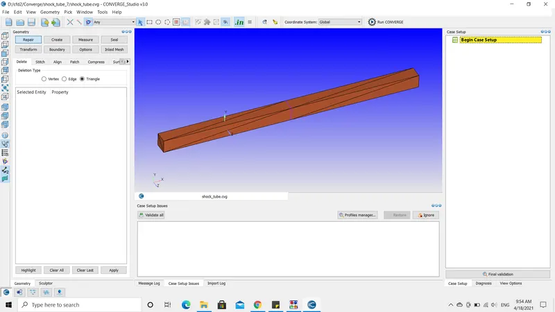
• First import the stl/cad file. Check for any error using the validation option.
• Later check the normal direction. If the normal arrows are directed outside the geometry transform them or change them to inside. This shows the direction of fluid flow.
• And begin the case setup.

----------------------------------------------------------------------------------------------------------------------------------------------------------------------------------------------------------------------------------------------------------------------------------------

Regions and Initialization:

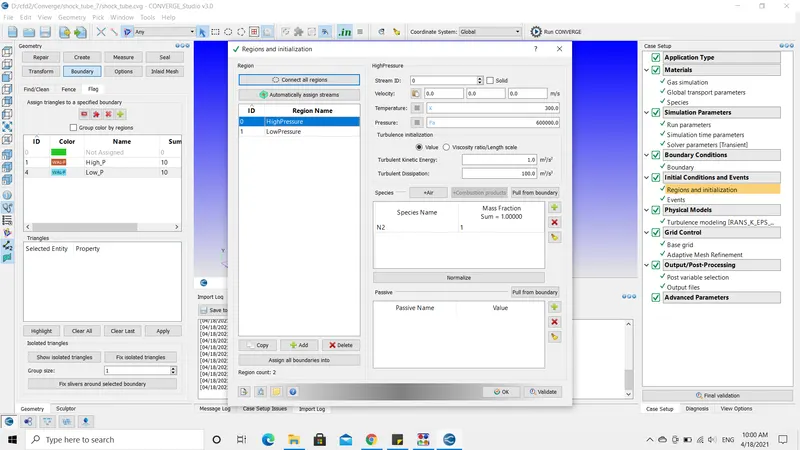
• After flagging the boundaries, set up the regions and by default, we do not get the events to option so add the events menu by clicking on the Initial Conditions option. It will open a dialogue box select the events option from there.
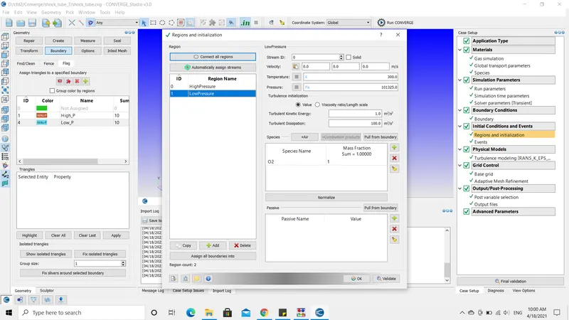
• In regions, we add two regions one for high-pressure and another for low-pressure.
• In high-pressure regions the conditions are pressure is equal to 6 bar, whereas in low-pressure the pressure is limited to atmospheric pressure.
• In high-pressure the fluid is N2 and for low-pressure, the fluid is O2 with a mass fraction of 1 each.

----------------------------------------------------------------------------------------------------------------------------------------------------------------------------------------------------------------------------------------------------------------------------------------

Boundary:

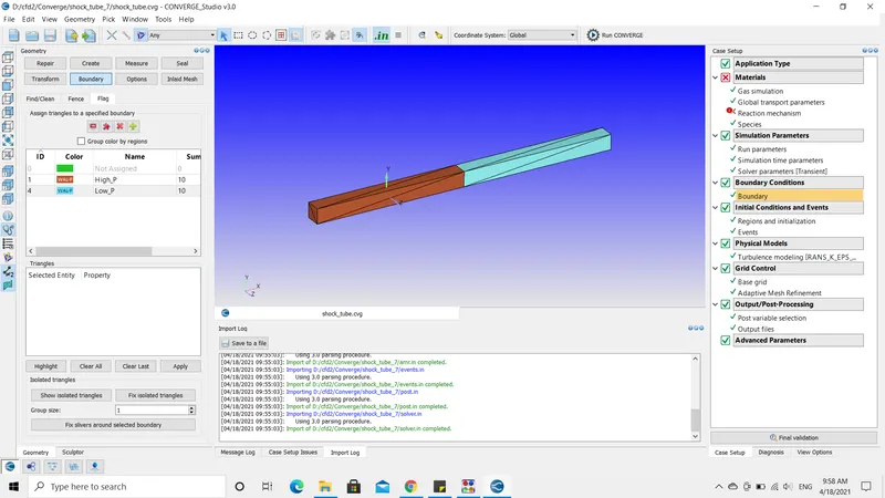
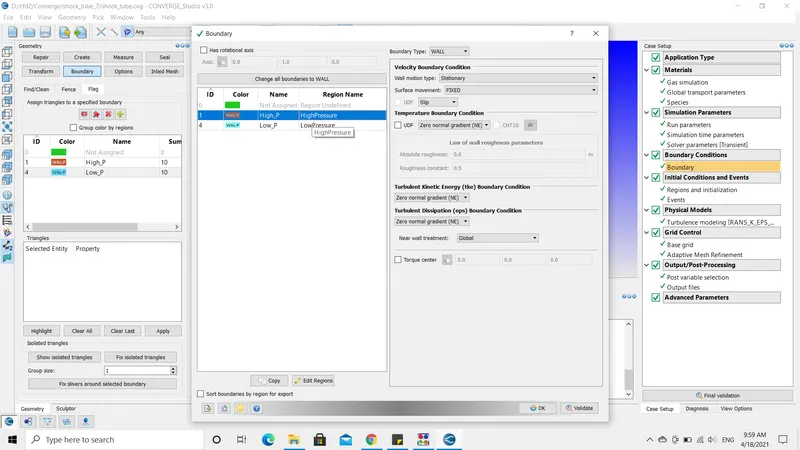
• If the geometry has zero errors after validating, proceed to flag the boundary as shown below.
• Here we have only boundaries high-pressure and low-pressure. After flagging, there will be 4 additional cells in between these two boundaries.
• To remove the extra cells, hide the low-pressure boundary and the unflagged boundary are visible there select them and press "D" on the keyboard to delete them(if the hotkey option is enabled in your software).

----------------------------------------------------------------------------------------------------------------------------------------------------------------------------------------------------------------------------------------------------------------------------------------

Regions and Initialization:

• After flagging the boundaries, set up the regions and by default, we do not get the events to option so add the events menu by clicking on the Initial Conditions option. It will open a dialogue box select the events option from there.
• In regions, we add two regions one for high-pressure and another for low-pressure.
• In high-pressure regions the conditions are pressure is equal to 6 bar, whereas in low-pressure the pressure is limited to atmospheric pressure.
• In high-pressure the fluid is N2 and for low-pressure, the fluid is O2 with a mass fraction of 1 each.

----------------------------------------------------------------------------------------------------------------------------------------------------------------------------------------------------------------------------------------------------------------------------------------

Events:

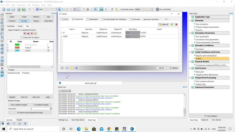
• As said at the beginning, there is a diaphragm introduced to stop the flow or exchange of fluids between the two regions. The events are used to open and close the diaphragm.

----------------------------------------------------------------------------------------------------------------------------------------------------------------------------------------------------------------------------------------------------------------------------------------

Materials:

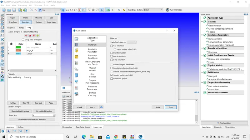
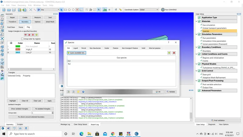
• Open the materials dialogue box and enable the species model and add Oxygen and Nitrogen in the species and shown in the second picture.

----------------------------------------------------------------------------------------------------------------------------------------------------------------------------------------------------------------------------------------------------------------------------------------

Simulation Parameters:

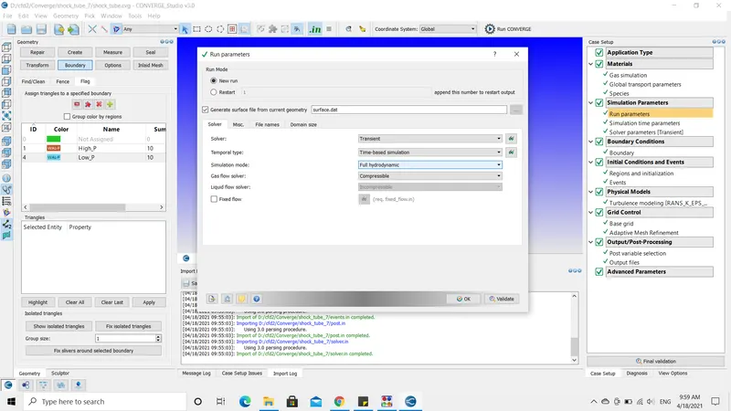
• Run Parameters: We are performing a transient case solver, accept the default values.

Simulation Time Parameter: For simulation time parameters the start time and end time are in seconds.

• The start time is zero as always and the end time would be 0.003 seconds.
• The initial time-step is 1e-09 second.
• Minimum time-step is 1e-09 second.
• Maximum time is 1 second.
• The CFL number is 1.

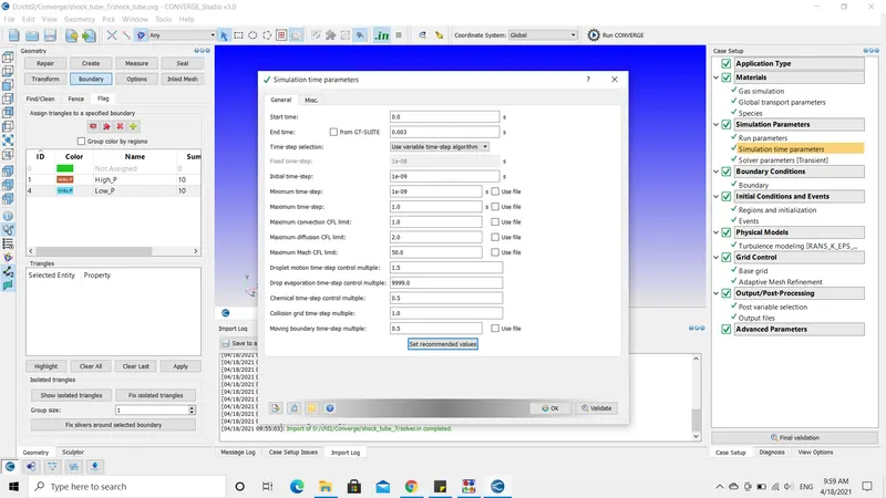
• For solver, parameters use default options and validate them for any errors.

----------------------------------------------------------------------------------------------------------------------------------------------------------------------------------------------------------------------------------------------------------------------------------------

Physical Models:

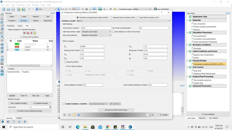
• I used the turbulence model and for the turbulence case, I used the k-Epsilon model with default values.

----------------------------------------------------------------------------------------------------------------------------------------------------------------------------------------------------------------------------------------------------------------------------------------

Grid Control:

• The size of the mesh of the grid is 0.001 meters.

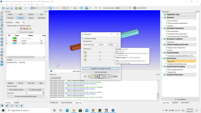
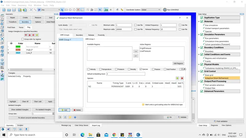
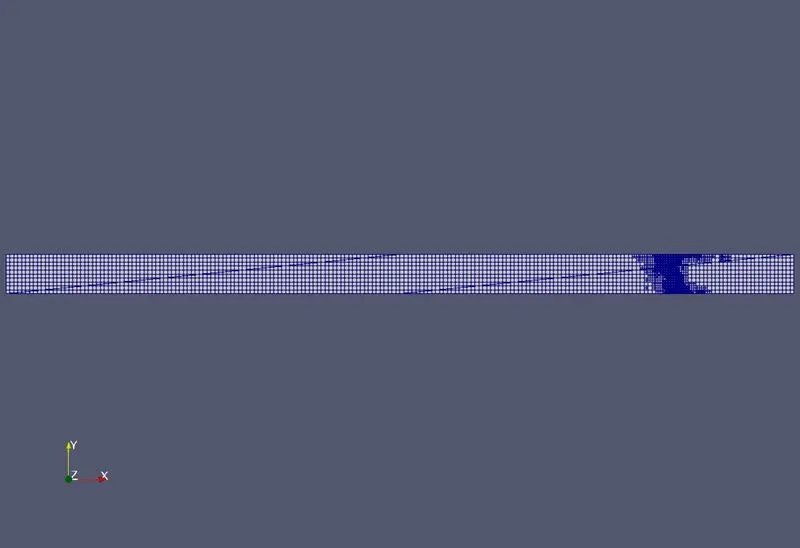
• I have also enabled the Adaptive Mesh Refinement method to check the species behaviors and the settings are displayed below.

----------------------------------------------------------------------------------------------------------------------------------------------------------------------------------------------------------------------------------------------------------------------------------------

PostProcessing:

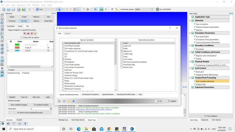
• Use the default options for the post variable selection.

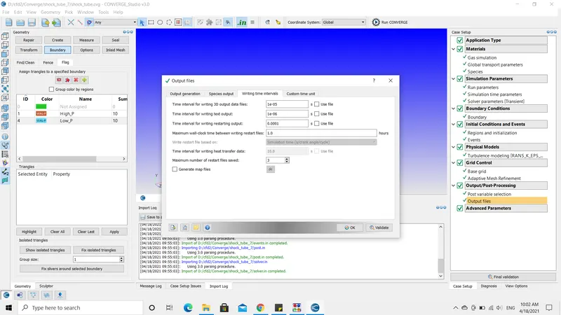
• Output files: The time interval for 3D output data files is 1e-05.

• Finally, validate the entire case setup, and if the errors are zero export the files and run the simulation using MPI setup.
• Later, convert the post files into ParaView format either by using convergent software or by MPI command.

----------------------------------------------------------------------------------------------------------------------------------------------------------------------------------------------------------------------------------------------------------------------------------------

Results:

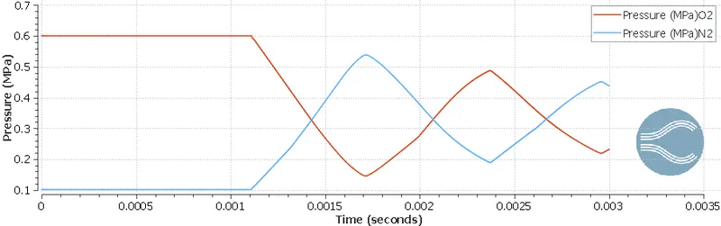
• Pressure Plot:

• Pressure Animation:

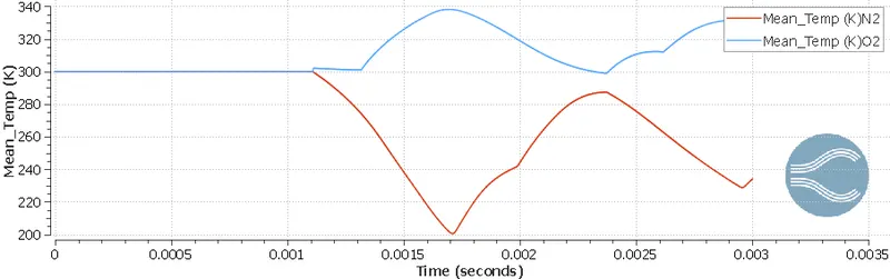
• Temperature Plot:

• Temperature Animation:

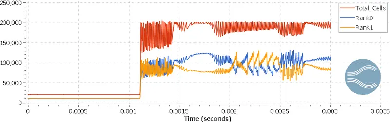
• Total Cell Count:

• Velocity Animation:

• Mesh:

CONCLUSION:

1. From the above simulation and results, we can study the characteristics of compressed gassed when it is introduced into a low-pressure region.
2. From the pressure animation, we can see that when the lid opened the high-pressure N2 gas enters into the low-pressure O2 region and try to compress the fluid and forms a recirculation.
3. Initially, the temperature is not stable after few seconds due to the sudden interaction of high-pressure and low-pressure gasses. Later the temperature attained an equilibrium position.
4. It is understandable from the above Pressure, Temperature, and Total Cell Count plots after 0.001 i.e., opening or removal of the diaphragm between two regions the characteristics are changing a lot.
5. This behaviour is due to the sudden escape of pressurised fluid in to the low-pressure cabin.
6. The mesh picture shows the AMR active regions where the species moment.