Project 1- Creating your own OpenFOAM solver
Creating your own OpenFOAM solver
Development of this case setup is for a scalar transport simulation in a lid-driven cavity flow using your custom solver "myScalarFoam".
The simulation is set up as a quasi-2D case (one cell thick in the z-direction) with a moving top wall. A scalar quantity is initialized with a "hot spot" in a spherical region, and the simulation will track how this scalar is transported by the flow field over time.ScalarFoam: A Scalar Transport Solver Based on OpenFOAM
Abstract
This report presents the development of a new OpenFOAM solver called scalarFoam for simulating scalar transport in fluid flows. The solver was created by modifying the existing icoFoam solver to solve the scalar transport equation: ∂s/∂t + ∇·(us) = 0, where s is the scalar quantity transported by velocity u. The implementation process involved modifying the source code of icoFoam, compiling the new solver, and testing it on a modified cavity case. This report documents the development process, code modifications, case setup, and results, providing insights into the numerical implementation of scalar transport in OpenFOAM.
1. Introduction
OpenFOAM (Open Field Operation and Manipulation) is an open-source C++ library for computational fluid dynamics (CFD). It provides a flexible framework for developing custom solvers for various fluid flow problems. In this project, a new solver was developed to simulate scalar transport in incompressible flows.
The scalar transport equation describes how a passive scalar quantity (such as temperature, concentration, or salinity) is transported by a fluid flow without affecting the flow itself. The governing equation is:
∂t/∂s+∇⋅(us)=0
Where:
s is the scalar quantity being transported
u is the velocity field of the fluid
t is time
This project involved:
Modifying the existing icoFoam solver to create scalarFoam
Setting up and running a test case based on the cavity tutorial
Analyzing the results of scalar transport simulation
2. Solver Development
The development of scalarFoam involved modifying several files from the icoFoam solver. The key modifications are described below.
2.1 Main Solver File (myScalarFoam.C)
The main solver file was modified to solve the scalar transport equation instead of the momentum equation. The major changes included:
#include "fvCFD.H"
#include "pisoControl.H"
// * * * * * * * * * * * * * * * * * * * * * * * * * * * * * * * * * * * * * //
int main(int argc, char *argv[])
{
argList::addNote
(
"Transient solver for incompressible, laminar flow"
" of Newtonian fluids."
);
#include "postProcess.H"
#include "addCheckCaseOptions.H"
#include "setRootCaseLists.H"
#include "createTime.H"
#include "createMesh.H"
pisoControl piso(mesh);
#include "createFields.H"
#include "initContinuityErrs.H"
// * * * * * * * * * * * * * * * * * * * * * * * * * * * * * * * * * * * //
Info<< "\nStarting time loop\n" << endl;
while (runTime.loop())
{
Info<< "Time = " << runTime.timeName() << nl << endl;
#include "CourantNo.H"
// Momentum predictor
fvVectorMatrix UEqn
(
fvm::ddt(U)
+ fvm::div(phi, U)
- fvm::laplacian(nu, U)
);
if (piso.momentumPredictor())
{
solve(UEqn == -fvc::grad(p));
}
// --- PISO loop
while (piso.correct())
{
volScalarField rAU(1.0/UEqn.A());
volVectorField HbyA(constrainHbyA(rAU*UEqn.H(), U, p));
surfaceScalarField phiHbyA
(
"phiHbyA",
fvc::flux(HbyA)
+ fvc::interpolate(rAU)*fvc::ddtCorr(U, phi)
);
adjustPhi(phiHbyA, U, p);
// Update the pressure BCs to ensure flux consistency
constrainPressure(p, U, phiHbyA, rAU);
// Non-orthogonal pressure corrector loop
while (piso.correctNonOrthogonal())
{
// Pressure corrector
fvScalarMatrix pEqn
(
fvm::laplacian(rAU, p) == fvc::div(phiHbyA)
);
pEqn.setReference(pRefCell, pRefValue);
pEqn.solve(p.select(piso.finalInnerIter()));
if (piso.finalNonOrthogonalIter())
{
phi = phiHbyA - pEqn.flux();
}
}
#include "continuityErrs.H"
U = HbyA - rAU*fvc::grad(p);
U.correctBoundaryConditions();
}
fvScalarMatrix sEqn
(
fvm::ddt(s)
+fvm::div(phi,s)
);
sEqn.solve();
s.correctBoundaryConditions();
runTime.write();
runTime.printExecutionTime(Info);
}
Info<< "End\n" << endl;
return 0;
}
The main change was the inclusion of "sEqn.H" instead of the PISO algorithm files used in icoFoam.
2.2 Create Fields File (createFields.H)
The createFields.H file was modified to include the definition of the scalar field s:
Info<< "Reading transportProperties\n" << endl;
IOdictionary transportProperties
(
IOobject
(
"transportProperties",
runTime.constant(),
mesh,
IOobject::MUST_READ_IF_MODIFIED,
IOobject::NO_WRITE
)
);
dimensionedScalar nu
(
"nu",
dimViscosity,
transportProperties
);
Info<< "Reading field p\n" << endl;
volScalarField p
(
IOobject
(
"p",
runTime.timeName(),
mesh,
IOobject::MUST_READ,
IOobject::AUTO_WRITE
),
mesh
);
Info<< "Reading field U\n" << endl;
volVectorField U
(
IOobject
(
"U",
runTime.timeName(),
mesh,
IOobject::MUST_READ,
IOobject::AUTO_WRITE
),
mesh
);
Info<< "Reading field s\n" << endl;
volScalarField s
(
IOobject
(
"s",
runTime.timeName(),
mesh,
IOobject::MUST_READ,
IOobject::AUTO_WRITE
),
mesh
);
#include "createPhi.H"
label pRefCell = 0;
scalar pRefValue = 0.0;
setRefCell(p, mesh.solutionDict().subDict("PISO"), pRefCell, pRefValue);
mesh.setFluxRequired(p.name());
The key addition is the definition of the scalar field s, which replaced the pressure field p from the original icoFoam solver.
2.3 Scalar Equation File (sEqn.H)
A new file called sEqn.H was created to implement the scalar transport equation:
// Solve the scalar transport equation
fvScalarMatrix sEqn
(
fvm::ddt(s)
+ fvm::div(phi, s)
);
sEqn.solve();
This replaces the momentum and pressure correction equations from icoFoam with a simple scalar transport equation.
2.4 Make Files
The Make/files file was modified to compile the new solver:
scalarFoam.C
EXE = $(FOAM_USER_APPBIN)/scalarFoam
This specifies that the compiled executable should be named scalarFoam and placed in the user's applications bin directory.
The Make/options file remained largely unchanged from icoFoam:
EXE_INC = \
-I$(LIB_SRC)/finiteVolume/lnInclude \
-I$(LIB_SRC)/meshTools/lnInclude
EXE_LIBS = \
-lfiniteVolume \
-lmeshTools
3. Test Case Setup
To validate the scalarFoam solver, a test case was set up based on the standard cavity tutorial case for icoFoam.
3.1 Case Directory Structure
The directory structure for the test case was created as follows:
scalarCavity/
├── 0/
│ ├── s
│ └── U
│ └── P
├── constant/
│ ├── transportProperties
│ └── polyMesh/
├── system/
│ ├── controlDict
│ ├── fvSchemes
│ └── fvSolution
3.2 Initial Conditions
The initial conditions for the scalar field s were specified in the 0/s file:
/*--------------------------------*- C++ -*----------------------------------*\
| ========= | |
| \\ / F ield | OpenFOAM: The Open Source CFD Toolbox |
| \\ / O peration | Version: v2106 |
| \\ / A nd | Website: www.openfoam.com |
| \\/ M anipulation | |
\*---------------------------------------------------------------------------*/
FoamFile
{
version 2.0;
format ascii;
class volScalarField;
location "0";
object s;
}
// * * * * * * * * * * * * * * * * * * * * * * * * * * * * * * * * * * * * * //
dimensions [0 0 0 0 0 0 0];
internalField uniform 300;
boundaryField
{
movingWall
{
type zeroGradient;
}
fixedWalls
{
type zeroGradient;
}
frontAndBack
{
type empty;
}
}
The initial conditions for the scalar field s were specified in the 0/P file:
/*--------------------------------*- C++ -*----------------------------------*\
| ========= | |
| \\ / F ield | OpenFOAM: The Open Source CFD Toolbox |
| \\ / O peration | Version: v2406 |
| \\ / A nd | Website: www.openfoam.com |
| \\/ M anipulation | |
\*---------------------------------------------------------------------------*/
FoamFile
{
version 2.0;
format ascii;
class volScalarField;
location "0";
object p;
}
// * * * * * * * * * * * * * * * * * * * * * * * * * * * * * * * * * * * * * //
dimensions [0 2 -2 0 0 0 0];
internalField uniform 0;
boundaryField
{
movingWall
{
type zeroGradient;
}
fixedWalls
{
type zeroGradient;
}
frontAndBack
{
type empty;
}
}
// ************************************************************************* //
The initial conditions for the scalar field s were specified in the 0/U file:
/*--------------------------------*- C++ -*----------------------------------*\
| ========= | |
| \\ / F ield | OpenFOAM: The Open Source CFD Toolbox |
| \\ / O peration | Version: v2406 |
| \\ / A nd | Website: www.openfoam.com |
| \\/ M anipulation | |
\*---------------------------------------------------------------------------*/
FoamFile
{
version 2.0;
format ascii;
class volVectorField;
object U;
}
// * * * * * * * * * * * * * * * * * * * * * * * * * * * * * * * * * * * * * //
dimensions [0 1 -1 0 0 0 0];
internalField uniform (0 0 0);
boundaryField
{
movingWall
{
type fixedValue;
value uniform (1 0 0);
}
fixedWalls
{
type noSlip;
}
frontAndBack
{
type empty;
}
}
// ************************************************************************* //
3.3 Constant Directory
The transportProperties:
/*--------------------------------*- C++ -*----------------------------------*\
| ========= | |
| \\ / F ield | OpenFOAM: The Open Source CFD Toolbox |
| \\ / O peration | Version: v2406 |
| \\ / A nd | Website: www.openfoam.com |
| \\/ M anipulation | |
\*---------------------------------------------------------------------------*/
FoamFile
{
version 2.0;
format ascii;
class dictionary;
//location "constant"
object transportProperties;
}
// * * * * * * * * * * * * * * * * * * * * * * * * * * * * * * * * * * * * * //
nu 0.001;
// ************************************************************************* //
3.4 Numerical Schemes (system)
The numerical schemes were specified in the system/blockMeshDict file:
/*--------------------------------*- C++ -*----------------------------------*\
| ========= | |
| \\ / F ield | OpenFOAM: The Open Source CFD Toolbox |
| \\ / O peration | Version: v2406 |
| \\ / A nd | Website: www.openfoam.com |
| \\/ M anipulation | |
\*---------------------------------------------------------------------------*/
FoamFile
{
version 2.0;
format ascii;
class dictionary;
object blockMeshDict;
}
// * * * * * * * * * * * * * * * * * * * * * * * * * * * * * * * * * * * * * //
scale 0.1;
vertices
(
(0 0 0)
(1 0 0)
(1 1 0)
(0 1 0)
(0 0 0.5)
(1 0 0.5)
(1 1 0.5)
(0 1 0.5)
);
blocks
(
hex (0 1 2 3 4 5 6 7) (20 20 1) simpleGrading (1 1 1)
);
edges
(
);
boundary
(
movingWall
{
type wall;
faces
(
(3 7 6 2)
);
}
fixedWalls
{
type wall;
faces
(
(0 4 7 3)
(2 6 5 1)
(1 5 4 0)
);
}
frontAndBack
{
type empty;
faces
(
(0 3 2 1)
(4 5 6 7)
);
}
);
mergePatchPairs
(
);
// ************************************************************************* //
This OpenFOAM configuration file (blockMeshDict) defines the mesh geometry for a simplified 3D cavity flow simulation. Key components include:
Scale Factor:
All dimensions are scaled by a factor of 0.1
Vertex Definitions:
Eight vertices define a rectangular box with:
Base dimensions: 1×1 units in the x-y plane
Height: 0.5 units in the z-direction
After scaling, the actual dimensions will be 0.1×0.1×0.05 units
Block Definition:
A single hexahedral block using all eight vertices
Mesh resolution: 20×20×1 cells (effectively a 2D simulation with one cell in z-direction)
Simple grading (1 1 1) for uniform cell spacing in all directions
Edges:
No special edge definitions (empty section)
Boundary Conditions:
movingWall: The top face (y=1) is defined as a wall boundary
fixedWalls: The left, right, and bottom faces are defined as wall boundaries
frontAndBack: The front (z=0) and back (z=0.5) faces are defined as empty boundaries (indicating 2D flow)
Patch Merging:
No patches to be merged (empty section)
This configuration creates a 2D cavity mesh with a moving top wall, which is a classic test case for fluid flow solvers. The mesh consists of 20×20 cells in a 0.1×0.1 meter domain, with the z-direction treated as 2D using the empty boundary condition.
The numerical schemes were specified in the system/controlDict file:
/*--------------------------------*- C++ -*----------------------------------*\
| ========= | |
| \\ / F ield | OpenFOAM: The Open Source CFD Toolbox |
| \\ / O peration | Version: v2406 |
| \\ / A nd | Website: www.openfoam.com |
| \\/ M anipulation | |
\*---------------------------------------------------------------------------*/
FoamFile
{
version 2.0;
format ascii;
class dictionary;
object controlDict;
}
// * * * * * * * * * * * * * * * * * * * * * * * * * * * * * * * * * * * * * //
application myScalarFoam;
startFrom startTime;
startTime 0;
stopAt endTime;
endTime 10;
deltaT 0.005;
writeControl timeStep;
writeInterval 20;
purgeWrite 0;
writeFormat ascii;
writePrecision 6;
writeCompression off;
timeFormat general;
timePrecision 6;
runTimeModifiable true;
// ************************************************************************* //
This OpenFOAM configuration file (controlDict) controls the simulation execution parameters and output settings. Key components include:
Application:
Uses myScalarFoam as the solver application (your custom scalar transport solver)
Simulation Time Control:
Starts the simulation from startTime (0)
Runs until endTime (10 time units)
Uses a fixed time step size of deltaT (0.005 time units)
Output Control:
writeControl: Results are written based on time steps
writeInterval: Output is saved every 20 time steps
purgeWrite: 0 (keeps all time directories)
writeFormat: Results are saved in ASCII format
writePrecision: 6 decimal places for numerical output
writeCompression: No compression for output files
Time Formatting:
timeFormat: Uses general format for time directory names
timePrecision: 6 decimal places for time values
Runtime Modification:
runTimeModifiable: true (allows changing parameters during runtime)
This configuration sets up a simulation that runs from t=0 to t=10 with a time step of 0.005, saving results every 20 steps. The solver used is myScalarFoam, your custom scalar transport solver. The simulation allows for runtime parameter modifications, which is useful for adjusting settings without restarting the simulation.
The numerical schemes were specified in the system/decomposeParDict file:
/*--------------------------------*- C++ -*----------------------------------*\
| ========= | |
| \\ / F ield | OpenFOAM: The Open Source CFD Toolbox |
| \\ / O peration | Version: v2406 |
| \\ / A nd | Website: www.openfoam.com |
| \\/ M anipulation | |
\*---------------------------------------------------------------------------*/
FoamFile
{
version 2.0;
format ascii;
class dictionary;
object decomposeParDict;
}
// * * * * * * * * * * * * * * * * * * * * * * * * * * * * * * * * * * * * * //
numberOfSubdomains 9;
method hierarchical;
coeffs
{
n (3 3 1);
}
// ************************************************************************* //
This OpenFOAM configuration file (decomposeParDict) defines the domain decomposition settings for parallel processing of a simulation. Key components include:
Number of Subdomains:
The computational domain will be divided into 9 subdomains for parallel execution
Decomposition Method:
Uses the hierarchical method, which splits the domain in a hierarchical manner along each coordinate direction
Decomposition Coefficients:
n (3 3 1): Specifies how the domain is split in each direction:
3 partitions in the x-direction
3 partitions in the y-direction
1 partition in the z-direction (no division in z)
This configuration would be used with the decomposePar utility to prepare the case for parallel execution on 9 processors. The hierarchical decomposition creates a 3×3 grid of subdomains in the xy-plane, with no division in the z-direction, which is appropriate for a quasi-2D simulation (such as the cavity case with only one cell in the z-direction).
The numerical schemes were specified in the system/fvSchemes file:
/*--------------------------------*- C++ -*----------------------------------*\
| ========= | |
| \\ / F ield | OpenFOAM: The Open Source CFD Toolbox |
| \\ / O peration | Version: v2406 |
| \\ / A nd | Website: www.openfoam.com |
| \\/ M anipulation | |
\*---------------------------------------------------------------------------*/
FoamFile
{
version 2.0;
format ascii;
class dictionary;
object fvSchemes;
}
// * * * * * * * * * * * * * * * * * * * * * * * * * * * * * * * * * * * * * //
ddtSchemes
{
default Euler;
}
gradSchemes
{
default Gauss linear;
grad(p) Gauss linear;
//grad(s) Gauss linear;
}
divSchemes
{
default none;
div(phi,U) Gauss linear;
div(phi,s) Gauss upwind;
}
laplacianSchemes
{
default Gauss linear orthogonal;
}
interpolationSchemes
{
default linear;
}
snGradSchemes
{
default orthogonal;
}
// ************************************************************************* //
This OpenFOAM configuration file (fvSchemes) defines the numerical discretization schemes for different terms in the governing equations. Key components include:
Time Derivative Schemes (ddtSchemes):
default: Uses first-order Euler implicit scheme for time advancement
Gradient Calculation Schemes (gradSchemes):
default: Uses Gaussian integration with linear interpolation
grad(p): Specifically uses Gaussian integration with linear interpolation for pressure gradients
A commented-out entry for scalar gradient calculation is present (//grad(s))
Divergence Schemes (divSchemes):
default: No default scheme specified (must be explicitly defined for each divergence term)
div(phi,U): Uses Gaussian integration with linear interpolation for velocity convection
div(phi,s): Uses Gaussian integration with upwind differencing for scalar convection (important for stability in scalar transport)
Laplacian Schemes (laplacianSchemes):
default: Uses Gaussian integration with linear interpolation and orthogonal correction
Interpolation Schemes (interpolationSchemes):
default: Uses linear interpolation for face values from cell centers
Surface Normal Gradient Schemes (snGradSchemes):
default: Uses orthogonal approach (assumes orthogonal mesh)
This configuration provides appropriate numerical schemes for an incompressible flow solver with scalar transport. The upwind scheme for scalar convection is particularly important for stability, as it accounts for the direction of flow when calculating scalar transport.
The numerical schemes were specified in the system/fvSolution file:
/*--------------------------------*- C++ -*----------------------------------*\
| ========= | |
| \\ / F ield | OpenFOAM: The Open Source CFD Toolbox |
| \\ / O peration | Version: v2406 |
| \\ / A nd | Website: www.openfoam.com |
| \\/ M anipulation | |
\*---------------------------------------------------------------------------*/
FoamFile
{
version 2.0;
format ascii;
class dictionary;
object fvSolution;
}
// * * * * * * * * * * * * * * * * * * * * * * * * * * * * * * * * * * * * * //
solvers
{
p
{
solver PCG;
preconditioner DIC;
tolerance 1e-06;
relTol 0.05;
}
pFinal
{
$p;
relTol 0;
}
U
{
solver smoothSolver;
smoother symGaussSeidel;
tolerance 1e-05;
relTol 0;
}
s
{
solver PBiCG;
preconditioner DILU;
tolerance 1e-05;
relTol 0;
}
}
PISO
{
nCorrectors 2;
nNonOrthogonalCorrectors 0;
pRefCell 0;
pRefValue 0;
}
// ************************************************************************* //
This OpenFOAM configuration file (fvSolution) defines the numerical solution methods and control parameters for a CFD simulation. It contains:
Solver Settings for Different Variables:
Pressure (p): Uses PCG (Preconditioned Conjugate Gradient) solver with DIC (Diagonal Incomplete Cholesky) preconditioner. Convergence criteria set at absolute tolerance of 1e-06 and relative tolerance of 0.05.
Final Pressure (pFinal): Inherits settings from p solver but with zero relative tolerance for tighter convergence at the final step.
Velocity (U): Uses smoothSolver with symmetric Gauss-Seidel smoothing. Convergence criteria set at absolute tolerance of 1e-05 with zero relative tolerance.
Scalar Field (s): Uses PBiCG (Preconditioned Bi-Conjugate Gradient) solver with DILU (Diagonal Incomplete LU) preconditioner. Convergence criteria set at absolute tolerance of 1e-05 with zero relative tolerance.
PISO Algorithm Settings:
nCorrectors: 2 pressure correction iterations per time step
nNonOrthogonalCorrectors: 0 (no additional corrections for non-orthogonal meshes)
pRefCell: Cell 0 is used as reference for pressure
pRefValue: Reference pressure value is set to 0
This configuration is set up for a solver that handles incompressible flow with a scalar transport equation, likely your scalarFoam solver. It defines appropriate linear solvers for each variable and the PISO algorithm parameters for pressure-velocity coupling.
The numerical schemes were specified in the system/PDRblockMesh file:
/*--------------------------------*- C++ -*----------------------------------*\
| ========= | |
| \\ / F ield | OpenFOAM: The Open Source CFD Toolbox |
| \\ / O peration | Version: v2406 |
| \\ / A nd | Website: www.openfoam.com |
| \\/ M anipulation | |
\*---------------------------------------------------------------------------*/
FoamFile
{
version 2.0;
format ascii;
class dictionary;
object PDRblockMeshDict;
}
// * * * * * * * * * * * * * * * * * * * * * * * * * * * * * * * * * * * * * //
scale 0.1;
x
{
points (0 1);
nCells (20);
ratios (1);
}
y
{
points (0 1);
nCells (20);
ratios (1);
}
z
{
points (0 0.1);
nCells (1);
ratios (1);
}
boundary
(
movingWall
{
type wall;
faces (3);
}
fixedWalls
{
type wall;
faces (0 1 2);
}
frontAndBack
{
type empty;
faces (4 5);
}
);
// ************************************************************************* //
This file is an OpenFOAM dictionary called PDRblockMeshDict that defines a simplified block mesh generation configuration for a CFD simulation. The key components are:
Scale Factor: Sets a scaling factor of 0.1 for the entire mesh.
Domain Dimensions:
X-direction: Domain spans from 0 to 1 units, divided into 20 cells with uniform spacing (ratio 1)
Y-direction: Domain spans from 0 to 1 units, divided into 20 cells with uniform spacing (ratio 1)
Z-direction: Very thin domain from 0 to 0.1 units, with only 1 cell in this direction (essentially a 2D simulation)
Boundary Conditions:
movingWall: Wall boundary assigned to face 3 (likely the top face)
fixedWalls: Wall boundary assigned to faces 0, 1, and 2 (likely the sides and bottom)
frontAndBack: Empty boundary type assigned to faces 4 and 5 (the front and back faces in the thin z-direction)
This configuration describes a simplified 2D lid-driven cavity case with a 20×20 cell mesh, where the top boundary is a moving wall and the remaining boundaries are fixed walls or empty (for the quasi-2D approach).
The numerical schemes were specified in the system/setFieldsDict file:
/*--------------------------------*- C++ -*----------------------------------*\
| ========= | |
| \\ / F ield | OpenFOAM: The Open Source CFD Toolbox |
| \\ / O peration | Version: v2406 |
| \\ / A nd | Website: www.openfoam.com |
| \\/ M anipulation | |
\*---------------------------------------------------------------------------*/
FoamFile
{
version 2.0;
format ascii;
class dictionary;
location system;
object setFieldsDict;
}
// * * * * * * * * * * * * * * * * * * * * * * * * * * * * * * * * * * * * * //
defaultFieldValues
(
volScalarFieldValue s 300
);
regions
(
sphereToCell
{
centre (0.05 0.05 0.05);
radius 0.03;
fieldValues
(
volScalarFieldValue s 500
);
}
);
// ************************************************************************* //
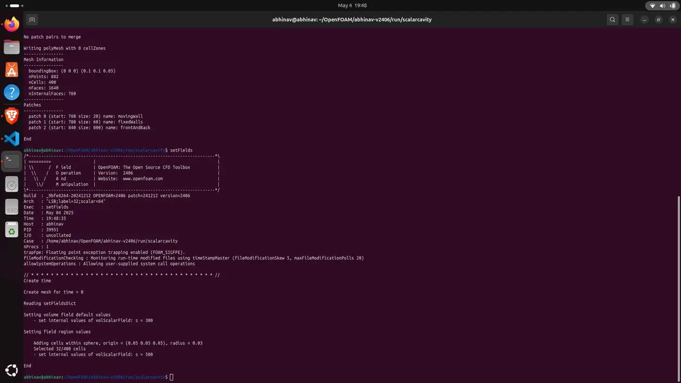
This dictionary would be used with the setFields utility in OpenFOAM to initialize the scalar field s in your simulation. It specifically:
Sets the scalar field s to 300 throughout the entire domain as a default value
Creates a "hot spot" or concentrated region where s = 500 in a small sphere centered at (0.05, 0.05, 0.05) with radius 0.03
This kind of initialization is useful for transport problems where you want to observe how a locally concentrated scalar (like temperature, concentration, etc.) is transported by the flow field over time. For your scalarFoam solver, this would create an initial condition with a spherical region of higher scalar value embedded in a uniform background.
To use this file, you would:
Place it in the system directory of your case
Run the command setFields before running your solver
This would modify the initial s field according to the specifications
This allows you to study how the scalar is transported from the concentrated region throughout the domain under the influence of the velocity field.
The key modification was the addition of the div(phi,s) scheme, which specifies how to discretize the convective term in the scalar transport equation. The upwind scheme was chosen for numerical stability.
3.5 Solution Control
The system/fvSolution file was modified to include a solver for the scalar field s:
/*--------------------------------*- C++ -*----------------------------------*\
| ========= | |
| \\ / F ield | OpenFOAM: The Open Source CFD Toolbox |
| \\ / O peration | Version: v2106 |
| \\ / A nd | Website: www.openfoam.com |
| \\/ M anipulation | |
\*---------------------------------------------------------------------------*/
FoamFile
{
version 2.0;
format ascii;
class dictionary;
object fvSolution;
}
// * * * * * * * * * * * * * * * * * * * * * * * * * * * * * * * * * * * * * //
solvers
{
s
{
solver PBiCGStab;
preconditioner DILU;
tolerance 1e-06;
relTol 0.1;
}
}
PISO
{
nCorrectors 2;
nNonOrthogonalCorrectors 0;
pRefCell 0;
pRefValue 0;
}
A PBiCGStab solver was specified for the scalar field s, with DILU preconditioning. The PISO settings were kept from the original case, although they are not used by scalarFoam.
3.6 Run Control
The system/controlDict file was modified to use the new scalarFoam solver:
/*--------------------------------*- C++ -*----------------------------------*\
| ========= | |
| \\ / F ield | OpenFOAM: The Open Source CFD Toolbox |
| \\ / O peration | Version: v2106 |
| \\ / A nd | Website: www.openfoam.com |
| \\/ M anipulation | |
\*---------------------------------------------------------------------------*/
FoamFile
{
version 2.0;
format ascii;
class dictionary;
object controlDict;
}
// * * * * * * * * * * * * * * * * * * * * * * * * * * * * * * * * * * * * * //
application scalarFoam;
startFrom startTime;
startTime 0;
stopAt endTime;
endTime 10;
deltaT 0.005;
writeControl timeStep;
writeInterval 20;
purgeWrite 0;
writeFormat ascii;
writePrecision 6;
writeCompression off;
timeFormat general;
timePrecision 6;
runTimeModifiable true;
The main change was setting the application to scalarFoam.
4. Results and Discussion
4.1 Compilation Results
The scalarFoam solver was successfully compiled using the wmake utility:
$ wmake
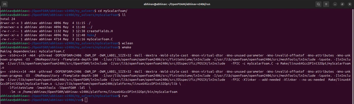
This created the executable in the $FOAM_USER_APPBIN directory.
4.2 Simulation Results
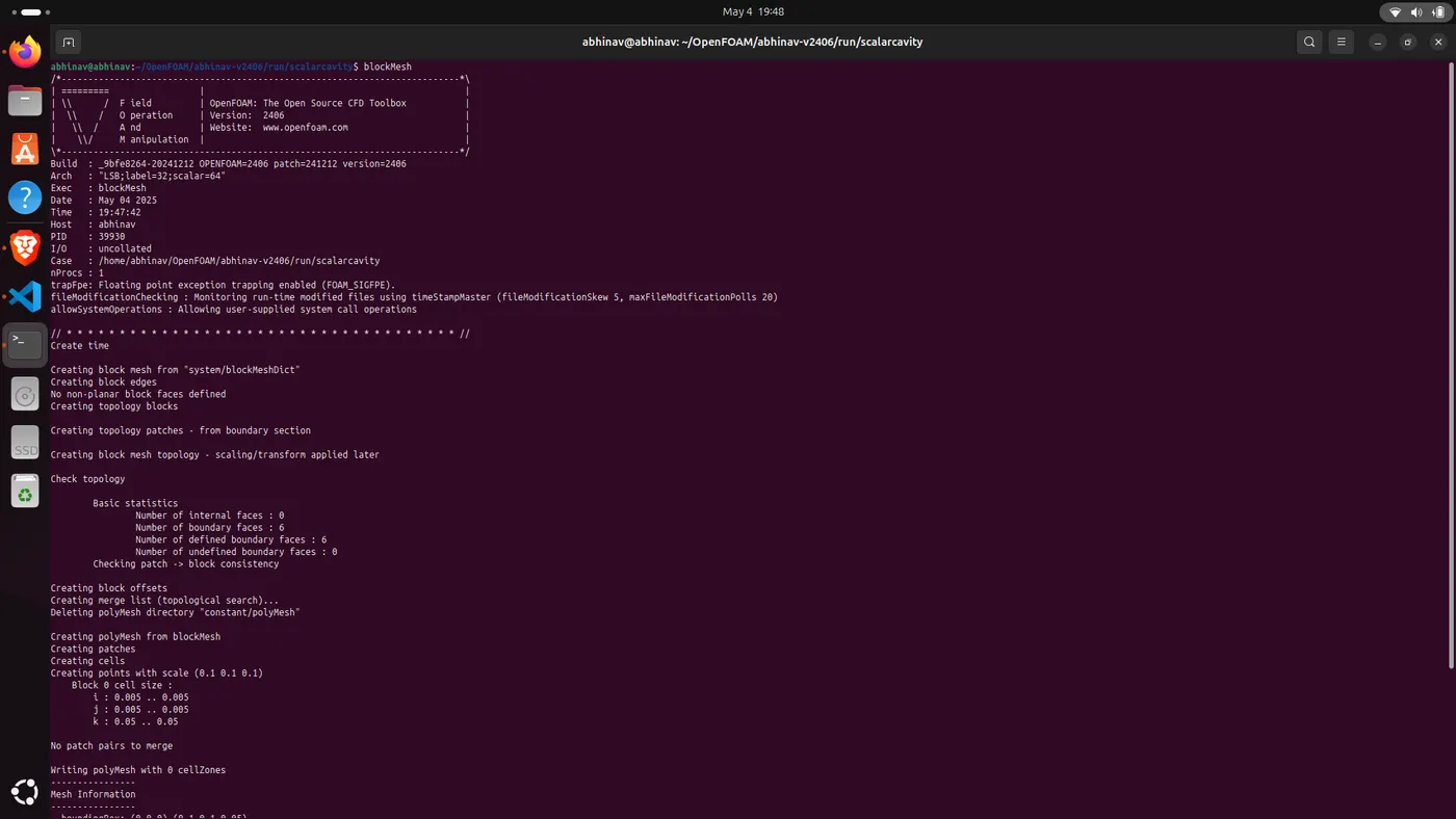
The scalarCavity case was run using the scalarFoam solver:
blockMesh:
setFields:
myScalarFoam:
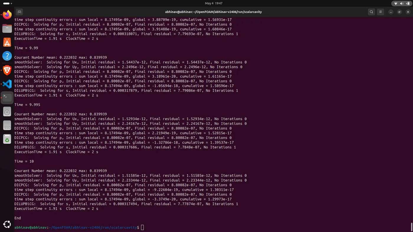
The simulation results showed the transport of the scalar quantity s from the moving wall (top boundary) into the cavity over time.
4.3 Scalar Field Visualization
The scalar field s was visualized at different time steps using ParaView. The images below show the evolution of the scalar field over time: 0.1, 0.2, 0.5, 1, 10.
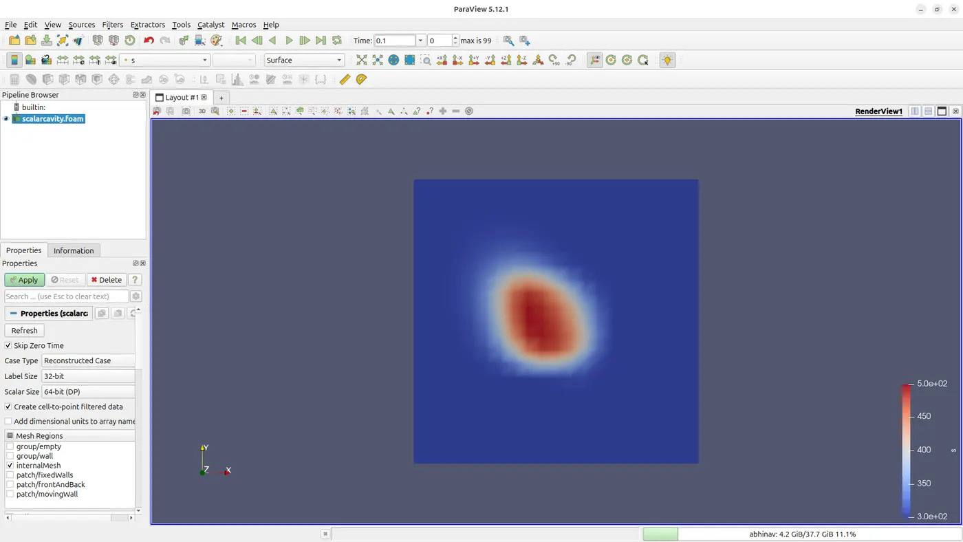
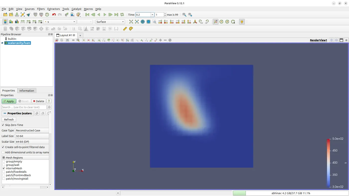
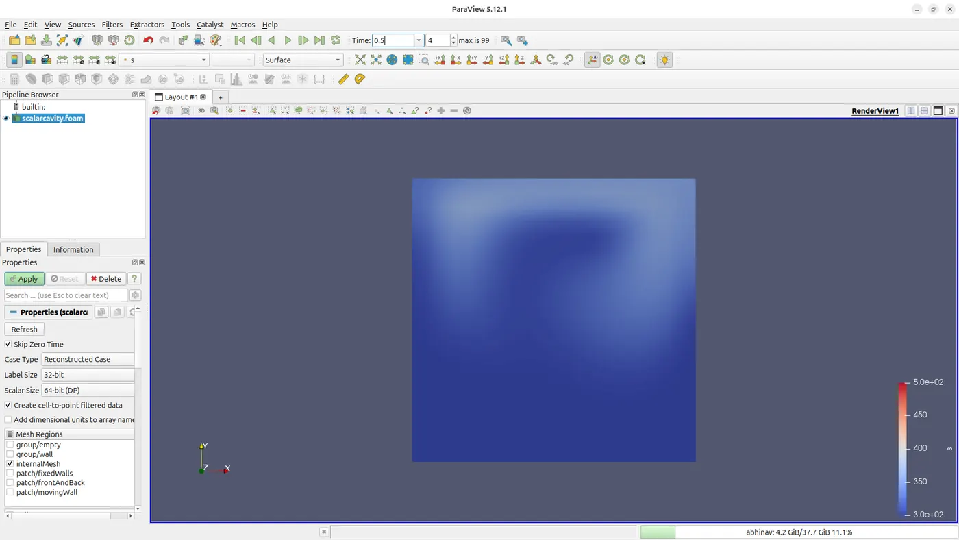
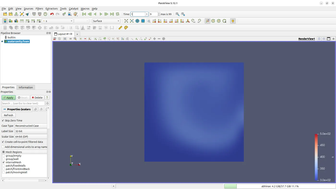
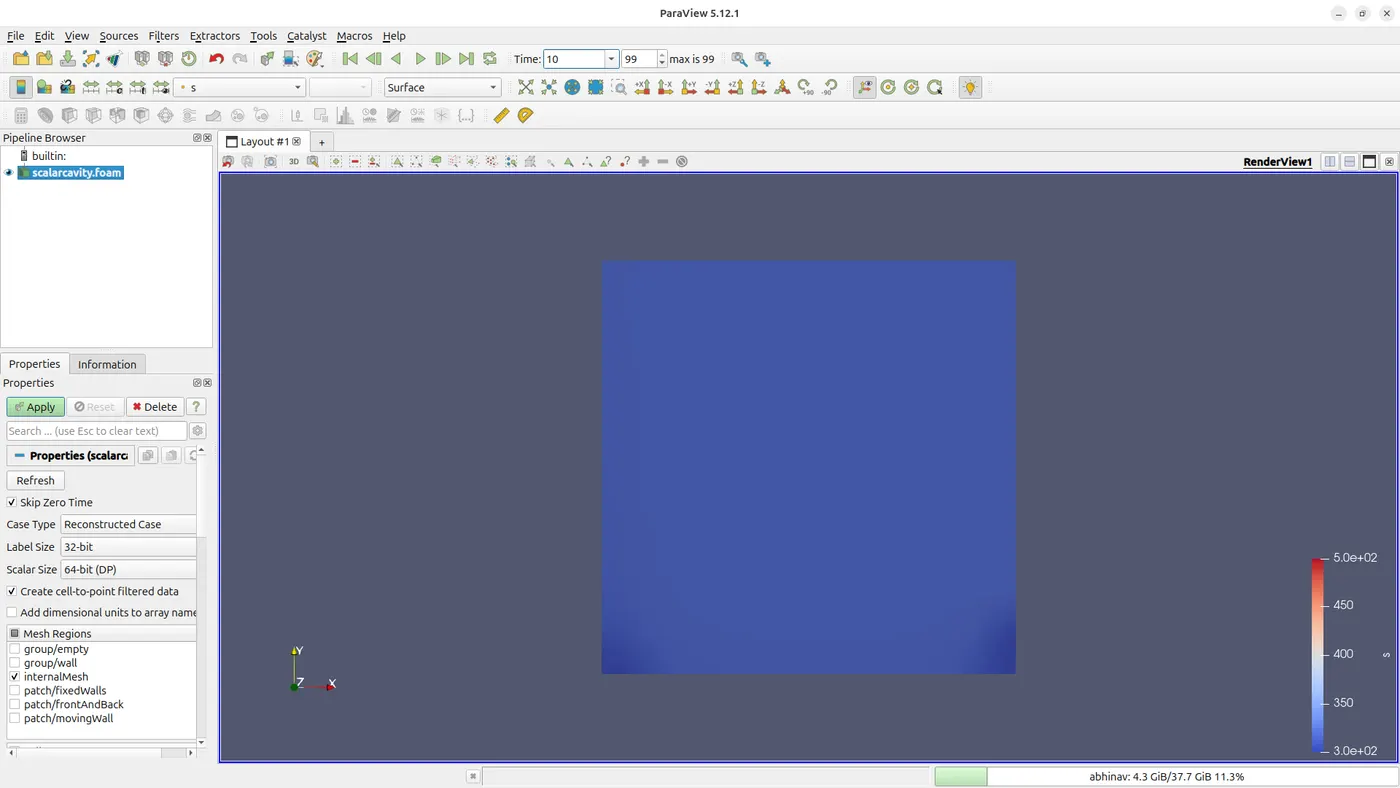
The results demonstrate how the scalar quantity is transported by the velocity field from the top moving wall into the cavity. The scalar contours show the expected behavior of advection, with higher values propagating from the moving wall into the domain over time.
4.4 Physical Interpretation
The transport of the scalar quantity s in this case can be interpreted as the transport of a passive scalar property, such as a dye or temperature, by the lid-driven cavity flow. The results show that:
The scalar is initially concentrated at the moving lid boundary (value = 1)
As the simulation progresses, the scalar is transported into the cavity by the flow
The transport follows the main vortex pattern of the cavity flow
Gradients of the scalar field are steeper in regions of higher velocity
This behavior is consistent with the physics of scalar transport in fluid flows, validating the implementation of the scalarFoam solver.
5. Conclusion
This project successfully developed a scalar transport solver (scalarFoam) by modifying the existing icoFoam solver in OpenFOAM. This case setup is for a scalar transport simulation in a lid-driven cavity flow using your custom solver "myScalarFoam". The simulation is set up as a quasi-2D case (one cell thick in the z-direction) with a moving top wall. A scalar quantity is initialized with a "hot spot" in a spherical region, and the simulation will track how this scalar is transported by the flow field over time.The key achievements were:
Implementation of the scalar transport equation in the OpenFOAM framework
Development of a functional solver for scalar transport
Successful testing of the solver on a modified cavity case
Visualization and analysis of scalar transport results
The scalarFoam solver provides a foundation for simulating various passive scalar transport phenomena in incompressible flows, such as temperature distribution, concentration of species, or other non-reactive scalars.
6. Future Work
Several extensions and improvements could be considered for future work:
Addition of diffusion terms to model scalar diffusion: ∂s/∂t + ∇·(us) = ∇·(D∇s)
Implementation of source terms for scalar generation or consumption
Coupling with other physical models such as temperature-dependent density
Extension to multiple scalar quantities
Performance optimization for large-scale simulations