Week 5: Prandtl Meyer Shock problem

AIM: To simulate a supersonic flow through a duct having a sharp corner to observe the formation of shock waves.

INTRODUCTION: In this simulation air with a velocity of 680 meters per second enters the duct. As soon as the air contacts the sharp corner the velocity increases and also the Mach Number increases while the static pressure, temperature, and density decrease.

THEORY:

Setting Up Geometry:

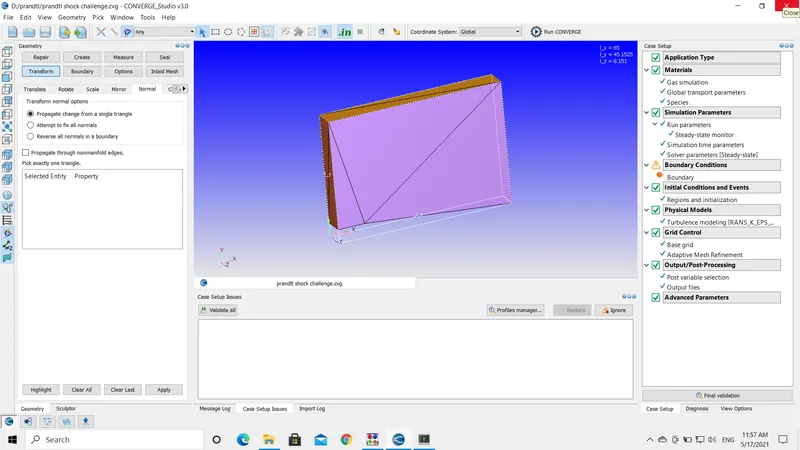
• For this simulation, the geometry is provided on the challenge page and I have uploaded the .STL file into the converge software.
• Initially, the geometry dimensions are in millimeters convert to meters by using the transform -> Scale option on the left-hand side tree.
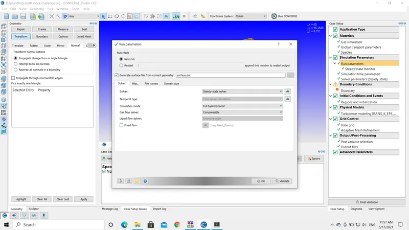
• I am using a Time-Based simulation.

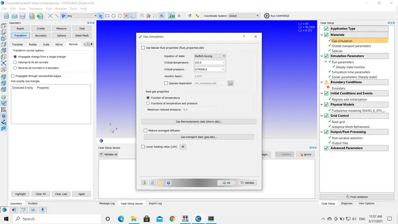
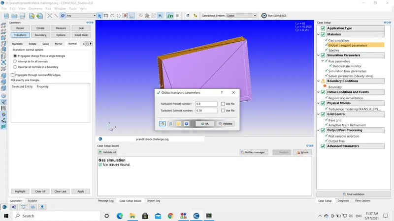
Gas Simulation & Global Transport Parameters:

• Choose the default options for both gas simulation and global parameters.

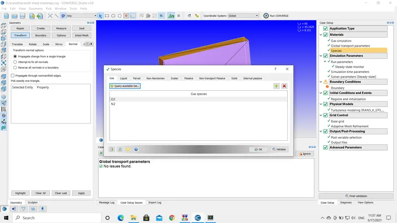
Species:

• Add new species in the species dialog box oxygen and nitrogen as shown below.

Run Parameters:

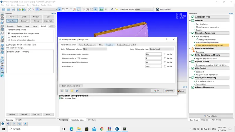
• I am using a steady-state solver with full-hydro simulation.
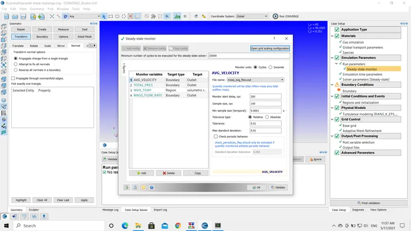
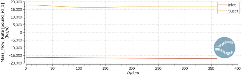
• I am monitoring the maximum temperature, total pressure, and mass flow rate at the outlet of the duct.
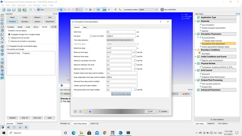
• I am running the simulation for 25000 cycles.

Boundary Conditions:

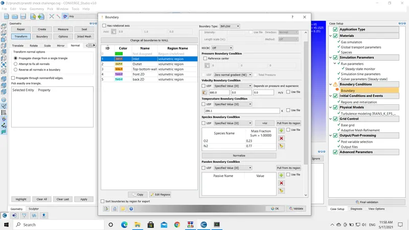
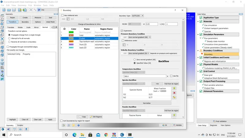
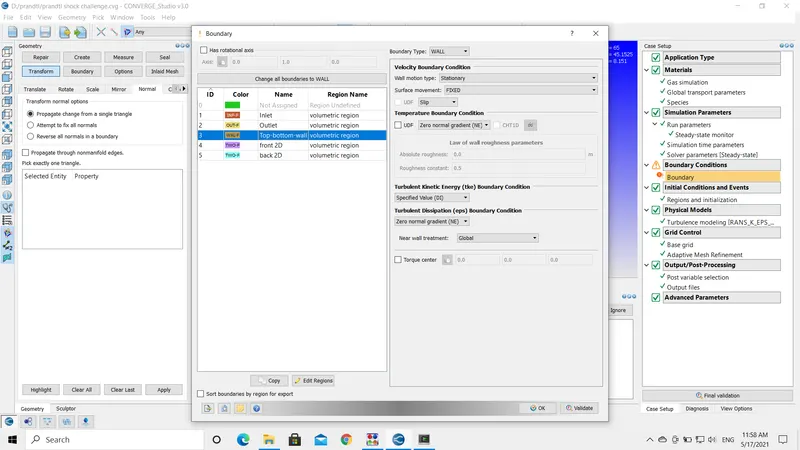
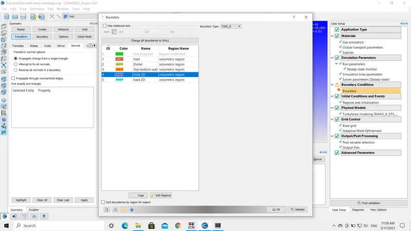
• The below mentioned pictures represent the values and conditions for the Inlet, Outlet, and Walls.
• The inlet velocity is 680 m/s and the pressure is set to NE condition.
• The outlet temperature is set to 300k and the fluid id set to be atmospheric air.

Regions and Initialization:

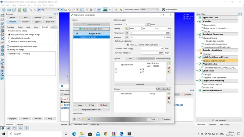
• For this setup, I have only one region, and atmospheric air with atmospheric pressure is mentioned in the region.

Physical Models:

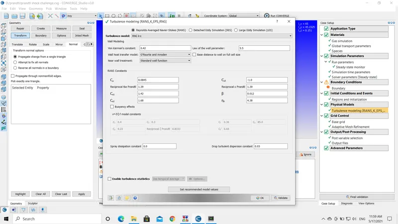
• I am using an RNG-K-epsilon turbulence model for this simulation.

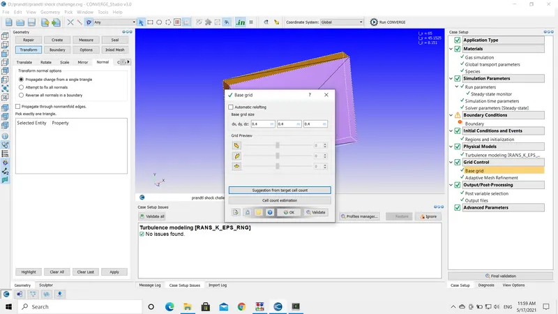
Grid Control:

Post Processing:

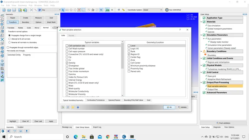
• Accept the default values for the post-processing.
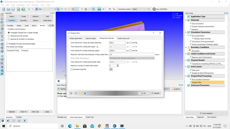
• And for output files, I am generating a 3D output file for every 250 cycles.

Results:

SGS 0.05:

Pressure Contour

Temperature Contour:

Velocity Contour:

SGS 0.1:

Pressure Contour:

Temperature Contour:

Velocity Contour:

Plots:

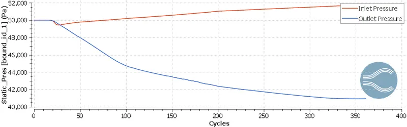
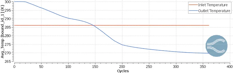
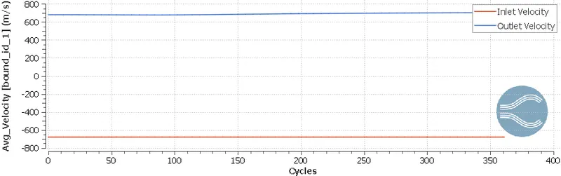
• SHOCK FLOW BOUNDARY CONDITION: For any boundary value problem the boundary condition constraints are necessary to complete the simulation. There are three main boundary conditions

1. Dirichlet Boundary Condition: This is also known as the first type of B.C. It is imposed on an ODE or PDE, the values are specified that the solution takes along the domain of the boundary.
2. Neumann Boundary Condition: This is also known as the second type of B.C. It is imposed on an ODE or PDE, the values are specified that the solution takes within the domain of the boundary.
3. Mixed Boundary Condition: In any given ODE or PDE that defines a boundary value problem to satisfy different types of boundary conditions on disjoint parts of the boundary of the domain where the conditions are stated.

• In simulations like shock flow, if the outlet pressure is assigned to be static and if the flow changes from subsonic to supersonic the given pressure conditions will no longer be valid and the pressure will be nullified from the flow in the interior. This is where the Neumann boundary condition is used. As the NE is dependent on the pressure and speed of air. These initial conditions (Pressure and Velocity) values are mentioned in the regions and initialization.

• SHOCK WAVE: A strong pressure wave in any elastic medium such as air, water, or a solid substance, produced by supersonic aircraft, explosions, lightning, or other phenomena that create violent changes in pressure. Shock waves differ from sound waves in that the wavefront, in which compression takes place, is a region of sudden and violent change in stress, density, and temperature. Because of this, shock acoustic waves. In particular, shock waves travel faster than sound, and their speed increases as the amplitude are raised: but the intensity of a shock wave also decreases faster than does that of a sound wave, because some of the energy of the shock wave is expended to heat the medium in which it travels. the amplitude of a strong strong shock wave, as created in the air by an explosion, decreases almost as the inverse square of the distance until the wave has become so weak that it obeys the laws of acoustic waves. Shock waves alter the mechanical, electrical, and thermal properties of solids and thus, can be used to study the equation of state of any material.

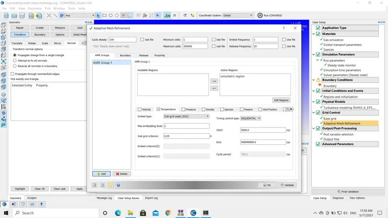
• Effect of SGS parameter on shock location: Subgrid scaling is an internal tool in Adaptive mesh refinement. This tool can be used for velocity, temperature, pressure, species and etc. In this simulation, I am using the temperature AMR with 0.1 and 0.05 SGS values. whenever the temperature value exceeds the specified SGS value the AMR will be activated in the region where there are abrupt changes.

Conclusion:

• I have uploaded all the results above, that are required to analyze.
• I have performed the analysis on SGS 0.1 and 0.05 and uploaded the results above for reference.
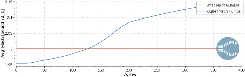
• After the air contacts, the corner the Mach number increases and this can be seen in the above plots.
• The plots also depict the expected trends, velocity and mass flow rate increases at the outlet and the pressure and temperature decreases
• However, the velocity mass flow rate increases due to the shock effect.
• Due to my software error, I could only convert 20 post files and demonstrate 350 cycles.