Week 3 - Taylor table method and Matlab code
Solving fourth-order approximation of the second derivative:
Central Difference
| Terms | f(i) | `triangle`xf'(x) | `triangle`xf''(x) | `triangle`xf'''(x) | `triangle`xf''''(x) | `triangle`xf'''''(x) | `triangle`xf''''''(x) |
| a*f*(i-2) | a | -2*a | 4*a/2 | -8*a/6 | 16*a/24 | -32*a/120 | 64*a/720 |
| b*f*(i-1) | b | -b | b/2 | -b/6 | b/24 | -b/120 | b/720 |
| c*f*(i) | c | 0 | 0 | 0 | 0 | 0 | 0 |
| d*f(i+1) | d | d | d/2 | d/6 | d/24 | d/120 | d/720 |
| e*f*(i+2) | e | 2*e | 4*e/2 | 8*e/6 | 16*e/24 | 32*e/120 | 64*e/720 |
| sum((af(i-2))+(bf(i-1))+(cf(1))+(df(i+1))+(ef(1+2))) | 0 | 0 | 1 | 0 | 0 | ? | ? |
The above equations are written as the following matrix.
A = [ 1 1 1 1 1
-2 -1 0 1 2
4 1 0 1 4
-8 -1 0 1 8
16 1 0 1 16]
B=[0
0
1
0
0]
X=[a1
b1
c1
d1
e1]
X_1=(A^-1)*B
a1= -0.0833;
b1= 1.3333;
c1=-2.5000;
d1= 1.3333;
e1= -0.0833;
Right-Sided Skewed DIfferencing
| Terms | f(i) | `triangle`xf'(x) | `triangle`xf''(x) | `triangle`xf'''(x) | `triangle`xf''''(x) | `triangle`xf'''''(x) | `triangle`xf'(x) |
|
a*f(i) |
a | 0 | 0 | 0 | 0 | 0 | 0 |
|
b*f(i+1) |
b | b | b/2 | b/6 | b/24 | b/120 | b/720 |
|
c*f(i+2) |
c | 2*c | 4*c/2 | 8*c/6 | 16*c/24 | 32*c/120 | 64*c/720 |
|
d*f(i+3) |
d | 3*d | 9*d/2 | 27*d/6 | 81*d/24 | 243*d/120 | 729*d/720 |
| e*f(i+4) | e | 4*e | 16*e/2 | 64*e/6 | 256*e/24 | 1024*e/120 |
4096*e/720 |
| f*f*(i+5) | f | 5*f | 25*f/2 | 125*f/6 | 625*f/24 | 3125*f/120 |
15625*f/720 |
|
sum((af(i))+bf(i+1)+ cf(i+2))+df(1+3)+ ef(i+4)+ff(i+5)) |
0 | 0 | 1 | 0 | 0 | 0 |
? |
A=[1 1 1 1 1
0 1 2 3 4
0 1/2 4/2 9/2 16/2
0 1/6 8/6 27/6 64/6
0 1/120 32/120 243/120 1024/120]
B=[0
0
1
0
0]
X=[a1
b1
c1
d1
e1]
X_2=(A^-1)*B_2
a2= 3.7500
b2=-12.8333
c2=17.8333
d2=-13.0000
e2=5.0833
f2-0.8333
- Left-Sided Skewed Differencing
| Terms | f(i) | `triangle`xf'(x) | `triangle`xf''(x) | `triangle`xf'''(x) | `triangle`xf''''(x) | `triangle`xf'''''(x) | `triangle`xf''''''(x) |
| a*f*(i) | a | 0 | 0 | 0 | 0 | 0 | 0 |
| b*f*(i-1) | b | -b | b/2 | -b/6 | b/24 | -b/120 | b/720 |
| c*f*(i-2) | c | -2*c | 4*c/2 | -8*c/6 | 16*c/24 | -32*c/120 | 64*c/720 |
| d*f*(i-3) | d | -3*c | 9*d/2 | -27*d/6 | 81*d/24 | -243*d/120 | 729*d/720 |
| e*f*(i-4) | e | -4*e | 16*e/2 | -64*e/6 | 256*e/24 | -1024*e/120 | 4096*e/720 |
| f*f*(i-5) | f | -5*f | 25*f/2 | -125*f/6 | 625*f/24 | -3125*f/120 | 15625*f/720 |
|
sum((af(i))+bf(i-1)+ cf(i-2)+df(1-3)+ef(i-4) +ff(i-5)) |
0 | 0 | 1 | 0 | 0 | 0 | ? |
A=[1 1 1 1 1
0 -1 -2 -3 -4
0 1/2 4/2 9/2 16/2
0 -1/6 -8/6 -27/6 -64/6
0 1/120 32/120 243/120 1024/120]
B_3=[0
0
1
0
0]
X=[a1
b1
c1
d1
e1]
X_3=(A^-1)*B_3
a=3 3.7500
b3=-12.8333
c3=17.8333
d3=-13.0000
e3=5.0833
f3=-0.8333
Through the above equations, I got central_differencing, Left_skewed_differencing, and Right_skewed_differencing values.
with those values, I have executed a program and plotted a loglog graph.
%fourth approximation central difference scheme.
%f(x)=exp(x)*cos(x);
clear all
close all
clc
% 1. Central difference
A_1=[1 1 1 1 1; -2 -1 0 1 2; 2 1/2 0 1/2 2; -8/6 -1/6 0 1/6 8/6; 16/24 1/24 0 1/24 16/24;];
% 2. Skewed right-sided difference
A_2=[1 1 1 1 1 1; 0 1 2 3 4 5; 0 1/2 2 9/2 8 25/2; 0 1/6 4/3 9/2 32/3 125/6; 0 1/24 2/3 27/8 32/3 625/24; 0 1/120 32/120 243/120 1024/120 3125/120];
% 3. Skewed left-sided difference
A_3=[1 1 1 1 1 1; 0 -1 -2 -3 -4 -5; 0 1/2 2 9/2 8 25/2; 0 -1/6 -4/3 -9/2 -32/3 -125/6; 0 1/24 2/3 27/8 32/3 625/24; 0 -1/120 -32/120 -243/120 -1024/120 -3125/120;];
%second-order derivative
B=[0; 0; 1; 0; 0];
B_2=[0; 0; 1; 0; 0; 0;];
B_3=[0; 0; 1; 0; 0; 0;];
%X=(A^-1)*B
X_1=inv(A_1)*B;
X_2=inv(A_2)*B_2;
X_3=inv(A_3)*B_2;
%fourth approximation central difference scheme.
%f(x)=exp(x)*cos(x);
x=pi/3;
dx=linspace(pi/4,pi/4000,15);
analytical_derivative=-2*exp(x)*sin(x);
%central differencing
for i=1:length(dx)
central_diff(i)=((X_1(1)*cos(x-2*dx(i))*exp(x-2*dx(i)))+(X_1(2)*cos(x-1*dx(i))*exp(x-1*dx(i)))+(X_1(3)*cos(x)*exp(x))+(X_1(4)*cos(x+1*dx(i))*exp(x+1*dx(i)))+(X_1(5)*cos(x+2*dx(i))*exp(x+2*dx(i))))/dx(i)^2;
right_skewed_diff(i)=((X_2(1)*cos(x)*exp(x))+(X_2(2)*cos(x+1*dx(i))*exp(x+1*dx(i)))+(X_2(3)*cos(x+2*dx(i))*exp(x+2*dx(i)))+(X_2(4)*cos(x+3*dx(i))*exp(x+3*dx(i)))+(X_2(5)*cos(x+4*dx(i))*exp(x+4*dx(i)))+(X_2(6)*cos(x+5*dx(i))*exp(x+5*dx(i))))/dx(i)^2;
left_skewed_diff(i) =((X_3(1)*cos(x)*exp(x))+(X_3(2)*cos(x-1*dx(i))*exp(x-1*dx(i)))+(X_3(3)*cos(x-2*dx(i))*exp(x-2*dx(i)))+(X_3(4)*cos(x-3*dx(i))*exp(x-3*dx(i)))+(X_3(5)*cos(x-4*dx(i))*exp(x-4*dx(i)))+(X_3(6)*cos(x-5*dx(i))*exp(x-5*dx(i))))/dx(i)^2;
central_error(i)=abs(central_diff(i)-analytical_derivative);
right_error(i)=abs(right_skewed_diff(i)-analytical_derivative);
left_error(i)=abs(left_skewed_diff(i)-analytical_derivative);
end
figure(1)
loglog(dx,central_error,'-ks','markerfacecolor','r')
hold on
loglog(dx,right_error,'-kd','markerfacecolor','b')
hold on
loglog(dx,left_error,'-ko','markerfacecolor','g')
hold on
grid on
hold off
xlabel('(dx)')
ylabel('Errors')
legend('Central Error','Right Side Error','Left Side Error')
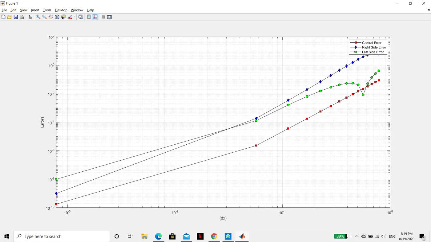
The above graph compares the errors between the three differences. It can be observed that central differencing has the least errors than left and right-skewed_differencing.
In other words, it can be expressed as central_differencing<Left_differencing<Right_differencing.