Week 5 - Mid term project - Solving the steady and unsteady 2D heat conduction problem

In this assignment, I am going to present the Steady and Unsteady 2D heat conduction problem.

For every heat conduction problem, there are certain initial and boundary conditions. The following are the conditions for the above problem.

The Top Temperature is 600K

The Bottom Temperature is 900K

The Left Temperature is 400K

The Right Temperature is 800K

The temperature values are stated in kelvin's

The governing equation we are using in this problem is a second-order partial differentiation. The steady-state method is a time-dependent

The other conditions are dt(Timestep), nx & ny(number of grid points), W(Omega), alpha, and CFL(Courant Fredrichs Lewy) Number.

Basically the CFL is observed in the unsteady heat conduction method and it is highly recommended that the CFL should be less than or equal to 0.5.

First: Steady-State 2D Heat Conduction

There are three types of heat transfer namely: Conduction, Convection, and Radiation.

Here we are going to discuss Conduction. Conduction is the transfer of energy i.e heat through a solid substance or material. 

The steady stated heat conduction equation is given as below:

`(del^2T)/(delx^2)` + `(del^2T)/(dely^2)`=0

`(del^2T)/(delx^2)`=`(T(i-1,j)-2T(i,j)+T(i+1,j))/(trianglex^2)`

`(del^2T)/(dely^2)`= `(T(i,j-1)-2T(i,j)+T(i,j+1))/(trianglex^2)`

`(T(i-1,j)-2T(i,j)+T(i+1,j))/(trianglex^2)`+`(T(i,j-1)-2T(i,j)+T(i,j+1))/(trianglex^2)`

since `Tp` = `T(i,j)`

and `K`=`(2(trianglex^2+triangley^2)/(trianglex^2*triangley^2))`

`Tp`=`(1/K)`*`(T(i-1,j)-2T(i,j)+T(i+1,j))/(trianglex^2)`+`(T(i,j-1)-2T(i,j)+T(i,j+1))/(trianglex^2)`

clear all
close all
clc

nx=10;
ny=10;
x=linspace(0,1,nx);
y=linspace(0,1,ny);
Y=fliplr(y);

dx=(x(2)-x(1));
dy=(y(2)-y(1));

T=ones(nx,ny);
T(1,:) = 600;
T(end,:) = 900;
T(:,1) = 400;
T(:,end) = 800;
Told=T;
error = 9e9;
tol=1e-5;

--------Here we are computing for jacobi solver---------

solver= 1;
tic
if solver==1
jacobi_iter=1;
while error>tol
for i=2:nx-1
for j=2:ny-1
term1=(Told(i+1,j)+Told(i-1,j))/(dx^2);
term2=(Told(i,j+1)+Told(i,j-1))/(dy^2);
k=2*((dx^2+dy^2)/(dx^2*dy^2));
T(i,j)=(term1+term2)/k;
end
end
error=max(max(abs(Told-T)));
Told=T;
jacobi_iter=jacobi_iter+1;
end
time1=toc;
figure(1)
colormap(jet)
contourf(x,Y,T,'showText','on')
tit1=sprintf('Jacobi Solver \n Number of Iterations=%d \n Iterations Time=%d S', jacobi_iter,time1);
title(tit1)
xlabel('X-axis');
ylabel('Y-axis');
colorbar
end

--------Here we are computing for Gauss Seidel solver---------

T=ones(nx,ny);
T(1,:) = 600;
T(end,:) = 900;
T(:,1) = 400;
T(:,end) = 800;
Told=T;
error = 9e9;
tol=1e-5;

solver=2;
tic
if solver==2
gauss_iter=1;
while error>tol
for i=2:nx-1
for j=2:ny-1
term1=(T(i-1,j)+Told(i+1,j))/(dx^2);
term2=(T(i,j-1)+Told(i,j+1))/(dy^2);
k=2*((dx^2+dy^2)/(dx^2*dy^2));
T(i,j)=(term1+term2)/k;
end
end
error=max(max(abs(Told-T)));
Told=T;
gauss_iter=gauss_iter+1;
end
time=toc;
figure(2)
colormap(jet)
contourf(x,Y,T,'showText','on')
tit1=sprintf('Gauss Solver \n Number of Iterations=%d \n Iterations Time=%d S', gauss_iter,time);
title(tit1)
xlabel('X-axis');
ylabel('Y-axis');
colorbar
end

--------Here we are computing for Successive Over Relaxation solver---------

T=ones(nx,ny);
T(1,:) = 600;
T(end,:) = 900;
T(:,1) = 400;
T(:,end) = 800;
Told=T;
error = 9e9;
tol=1e-5;

solver=3;
W=1.5;
tic
if solver==3
sor_iter=1;
while error>tol
for i=2:nx-1
for j=2:ny-1
term1=(T(i-1,j)+Told(i+1,j))/(dx^2);
term2=(T(i,j-1)+Told(i,j+1))/(dy^2);
% k=2*((dx^2+dy^2)/(dx^2*dy^2));
T(i,j)=Told(i,j)*(1-W)+W*((term1+term2)/k);
end
end
error=max(max(abs(Told-T)));
Told=T;
sor_iter=sor_iter+1;
end
time2=toc;
figure(3)
colormap(jet)
contourf(x,Y,T,'showText','on')
tit1=sprintf('SOR Solver \n Number of Iterations=%d \n Iterations Time=%d S', sor_iter,time2);
title(tit1)
xlabel('X-axis');
ylabel('Y-axis');
colorbar
end

Results:

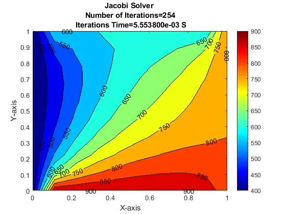
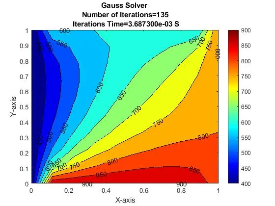
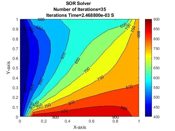
Conclusion:  

1. From the above pictures, it can be said that the temperature profile (Steady state) for Jacobi, Gauss, and SOR iterative methods are similar but the time is taken to converge the solution and the number of iterations is different for each iterative method.
2. In my solution, the Jacobi method has higher iterations than Gauss-Seidel and SOR(Successive Over Relaxation) has the least number of iterations than the other two methods.
3. The simulation time/Iterations time is Jacobi>Gauss>SOR.
4. In the SOR method, the relation factor plays a major role in converging the solution. It is important to have a close observation of the relaxation factor i.e, omega(W). This can reduce simulation time and iteration values.

 -------------------------------------------------------------------------------------------------------------

Unsteady State Heat Conduction(Explicit):

`(delT)/(delt)=alpha((del^2T)/(delx^2)+(del^2T)/(dely^2))`

`T(i,j)^(n+1)=T(i,j)^n+k1(T(i-1,j))-2T(i,j)+T(i+1,j))^n+k2(T(i,j-1))-2T(i,j)+T(i,j+1))`

Since `alpha`= thermal diffusivity

`k1=alpha*(delT)/(delx^2)`

`k2=alpha*(delT)/(dely^2)`

clear all
close all
clc

nx=10;
ny=10;
x=linspace(0,1,nx);
y=linspace(0,1,ny);

Y=fliplr(y);
dx=(x(2)-x(1));
dy=(y(2)-y(1));
dt=0.001;
alpha=3.1;

T = ones(nx,ny);
T(1,:)= 600; %temperature top in kelvins
T(end,:)=900;%temperature bottom
T(:,1)=400; %temperature left
T(:,end)=800; %temperatur right

Told=T;

error=9e9;
tol=1e-5;
k1=alpha*(dt/dx^2);
k2=alpha*(dt/dy^2);

cfl=k1+k2;
explicit_solver=1;
explicit_iter=1;
tic
if explicit_solver==1
while error>tol
for i=2:nx-1
for j=2:ny-1
term1=(Told(i-1,j)+Told(i+1,j)-2*Told(i,j))*k1;
term2=(Told(i,j-1)+Told(i,j+1)-2*Told(i,j))*k2;
T(i,j)=(Told(i,j)+term1+term2);
end
end
error=max((max(abs(Told-T))));
Told=T;
explicit_iter=explicit_iter+1;
end
figure(1)
time=(toc);
colormap(jet)
contourf(x,Y,T,'showText','on')
titl=sprintf('Explicit Method \n Number of Iterations=%d \n Simulation Time=%d \n',explicit_iter,time);
title(titl)

xlabel("X-Axis");
ylabel("Y-Axis");
colorbar
pause(0.03)
end

---------------------Explicit Image----------------

 

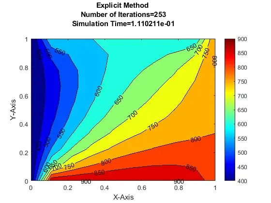
Conclusion:

1. The above picture represents the transient explicit method. This is similar to the steady-state solution.
2. In the transient method, we do not use Jacobi, Gauss, or SOR method. As we are finding the N'th order.
3. I have made a trial and error method for dt and courant values to get the optimum solution, finally  

---------------------Implicit Method---------------

Unsteady State Heat Conduction(Implicit):

`(delT)/(delt)=alpha((del^2T)/(delx^2)+(del^2T)/(dely^2))`

`T(i,j)^(n+1)=T(i,j)^n+k1(T(i-1,j)^(n+1)-2T(i,j)^n+T(i+1,j)^(n+1))+k2(T(i,j-1)^(n+1)-2T(i,j)^n+T(i,j+1)^(n+1))`

Since `alpha`= thermal diffusivity

`k1=alpha*(delT)/(delx^2)`

`k2=alpha*(delT)/(dely^2)`

close all
clear all
clc

nx=10;
ny=10;
x=linspace(0,1,nx);
y=linspace(0,1,ny);
Y=fliplr(y);
dx=(x(2)-x(1));
dy=(y(2)-y(1));

alpha=3.1;
dt=0.001;

k1=(alpha*dt)/(dx^2);
k2=(alpha*dt)/(dy^2);
nt=150;
CFL1=k1+k2;

T=ones(nx,ny);
T(1,:) =600;
T(end,:) =900;
T(:,1) =400;
T(:,end) =800;

Told=T;
Tinit=Told;

error=9e9;
tol=1e-5;

implicit_solver=1;

tic
if implicit_solver==1
jacobi_iter=1;
for k=1:nt
error=1;
while error>tol
for i=2:nx-1
for j=2:ny-1
term1=(Told(i-1,j)+Told(i+1,j))*k1;
term2=(Told(i,j-1)+Told(i,j+1))*k2;
T(i,j)=(Tinit(i,j)+(term1)+(term2))/(1+2*(k1+k2));
end
end
error=max(max(abs(Told-T)));
Told=T;
jacobi_iter=jacobi_iter+1;
end
Tinit=T;

end
time1=toc;
figure(1)
colormap(jet)
contourf(x,Y,T,'showText','on')
tit1=sprintf('Implicit Jacobi Method \n Number of iteration=%d\n Simulation time=%d s' ,jacobi_iter,time1);
title(tit1)

xlabel("X-Axis");
ylabel("Y-Axis");
colorbar
pause(0.3)
end

T=ones(nx,ny);
T(1,:) =600;
T(end,:) =900;
T(:,1) =400;
T(:,end) =800;

Told=T;
Tinit=Told;
Tupd=T;
k1=(alpha*dt)/(dx^2);
k2=(alpha*dt)/(dy^2);
CFL2=k1+k2;
error=9e9;
tol=1e-5;

implicit_solver=2;
tic
if implicit_solver==2
gauss_iter=1;
Tupd=T;
for k=1:nt
error=1;
while error>tol
for i=2:nx-1
for j=2:ny-1
term3=(Tupd(i-1,j)+Tupd(i+1,j))*k1;
term4=(Tupd(i,j-1)+Tupd(i,j+1))*k2;
T(i,j)=(Tinit(i,j)+(term3)+(term4))/(1+2*(k1+k2));
Tupd=T;
end
end
error=max(max(abs(Told-T)));
Told=T;
gauss_iter=gauss_iter+1;
end
Tinit=T;
end
time2=toc;
figure(2)
colormap(jet)
contourf(x,Y,T,'showText','on')
tit2=sprintf('Implicit Gauss Method \n Number of iteration=%d\n Simulation time=%d s' ,gauss_iter,time2);
title(tit2)

xlabel("X-Axis");
ylabel("Y-Axis");
colorbar
pause(0.3)
end

W=1.19;

T=ones(nx,ny);
T(1,:) =600;
T(end,:) =900;
T(:,1) =400;
T(:,end) =800;

Told=T;
Tinit=Told;
Tupd=T;
k1=(alpha*dt)/(dx^2);
k2=(alpha*dt)/(dy^2);
CFL3=k1+k2;
error=9e9;
tol=1e-5;

implicit_solver=2;
tic
if implicit_solver==2
sor_iter=1;
Tupd=T;
for k=1:nt
error=1;
while error>tol
for i=2:nx-1
for j=2:ny-1
term3=(Tupd(i-1,j)+Tupd(i+1,j))*k1;
term4=(Tupd(i,j-1)+Tupd(i,j+1))*k2;
T(i,j)=W*(Tinit(i,j)+(term3)+(term4))/(1+2*(k1+k2))+(1-W)*Told(i,j);
Tupd=T;
end
end
error=max(max(abs(Told-T)));
Told=T;
sor_iter=sor_iter+1;
end
Tinit=T;
end
time3=toc;
figure(3)
colormap(jet)
contourf(x,Y,T,'showText','on')
tit2=sprintf('Implicit SOR Method \n Number of iteration=%d\n Simulation time=%d s' ,sor_iter,time3);
title(tit2)

xlabel("X-Axis");
ylabel("Y-Axis");
colorbar
pause(0.3)
end

 

 

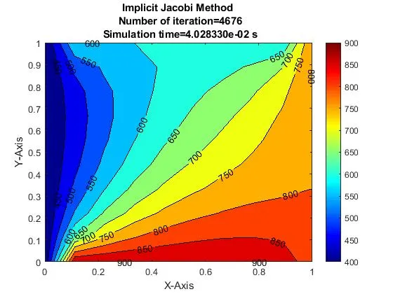
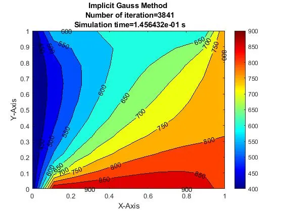
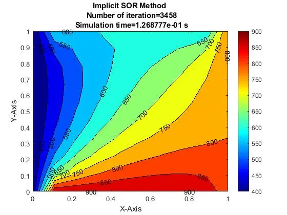
 Conclusion:

1.  For a particular value of time step(dt), W(omega/relaxation factor), and alpha, all three solvers plotted the same output.
2. In my case the time for iterations Gauss>SOR>Jacobi. But the iteration values Jacobi>Gauss>SOR. Jacobi method has the least simulation time but higher iteration values.

Overall conclusion:

1. In this project, steady and transient 2D heat conduction gave similar solutions so we could conclude that the transient method could be utilized for problems like this. Because it consumes very little time compared to other methods.
2. Iteration time/Simulation time for SOR is the least steady-state method but it is higher in Unsteady heat conduction this is due to the relaxation factor and CFL values and also the time marching value we give before the loop.
3. In unsteady heat conduction, the implicit and explicit doesn't yield a sable output unless the CFL number is less than or equal to 0.5.
4. I have observed one more thing, the iteration values also depend on the number of grids i.e, nx, and ny values. 
5. you may have noticed my alpha value is greater in implicit than in the explicit or steady-state.  This is due to the courant number and timestep just to make my plottings look converged.