Exhaust Port Challenge

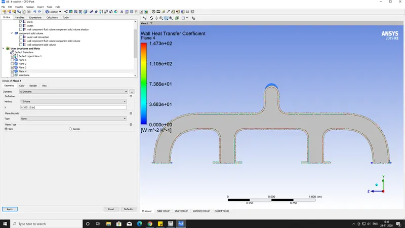
Aim: The main aim of this challenge is to observe the behavior of the coefficient of heat transfer through the outlet valve using the wall heat transfer coefficient in CFX post-processing.

Introduction: In this challenge, we have taken an exhaust port that represents a 4 cylinder engine with one outlet i.e, we have four inlets and one outlet. The inlet temperature is 700k and the velocity is 5 m/s.

The fluid flow is chosen to be turbulent and we have two options for this k-epsilon and k-omega. In future points, I will mention the approximate values and correct turbulent method for this type of analysis.

• To start the fluent simulation first, we begin with the geometry setup. In addition to the solid volume, we have to create fluid volume to calculate and observe the fluid flow and temperature characteristics in different regions of the pipes.
• The fluid volume is created using the volume extract option in the "prepare" tab. This looks as below shown picture.

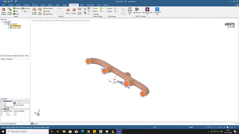
• Next, we assign the topology of the geometry to share, and at the inlet region, both the circles of solid and fluid dimensions must collide. To match the dimensions go to "workbench" and select the share option and click on the green tick button to start the operation. This will remove all the errors and align the dimensions.
• Moving to the meshing section, set the element size as small as possible to get a smooth simulation output. Introduce the sizing at Inlet and entire body.
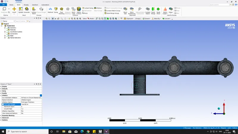
• To maintain the Y+ enable the inflation layer and choose the first layer thickness option and give the proper first layer height layer value.
• Lastly, in the meshing section name the boundaries.
• In the fluent setup, we have two materials, solid and fluid material. For solid we choose aluminum and for fluid, we select the default air material.
• Make sure to enable the energy equation on. The temperature and inlet velocity is mentioned at the beginning.

Theory:

I will demonstrate the difference between the two viscous methods and which is apt to this type of analysis.

• Although both are turbulent modeling solvers there is a minute difference between them they are semi-analytic models.
• K-epsilon model predicts the values far away from the boundaries/walls/surfaces. Whereas, K-omega model gives the values closest to the boundaries/walls/surfaces.
• Both models are dependent on the Y+ value. The Y+ range for k-epsilon and K-omega is different.
• For K-Omega the range is 1-5 and for K-epsilon the range is 30-300.

Objectives of this challenge:

• 1) Firstly, CHT stands for Conjugate Heat Transfer. The CHT analysis is used to describe the process that involves a change of temperature between solids and fluids. This change is due to the thermal energy between two physical bodies which is also known as "The Study of Heat Transfer".
• There are three types of heat transfer Conduction, Convection, and Radiation.
• As mentioned above CHT involves in exchange of temperature between solids and fluids. In solids, conduction is always greater whereas in fluids convection is greater.
• Whenever mechanical designs such as 4 stroke engines, exhaust pipe, heat sinks, turbines, nuclear generators, etc. They experience typical problems like heat transfer coefficient, temperature distribution, temperature response in certain areas where there is a time limit (vehicle engine cooling).
• The above mentioned are some of the areas where conjugate heat transfer analysis is important to improve the life of the machine for a long period of time.
• Conjugate Heat Transfer analysis can be used to improve the cooling performance of the water jacket and increase engine life. Advancements in cooling for applications such as gas turbine components require an improved understanding of the complex heat transfer mechanisms and the interactions between those mechanisms, which our engineers can perform without hassle.
• Critical cooling applications often rely on multiple thermal protection techniques, including internal cooling, external film cooling, etc. which are efficiently used by our analysis to cool components and limit the use of coolant. we do extensive support for motor and battery CHT analysis to get an optimized design for high voltage systems.
• Results of CHT analysis become the input to structural simulations as thermal loads.

2) Y+ Calculations

`Y+=(Y*u_t)/v`

`u_t =sqrt(tau_w/rho)`

`tau_w=0.5*c_f*rho*u^2`

`c_f=0.0576*Re^-0.2`

`Re=(rho*v*l)/(mu)`

• As we know that the Y+ values are different for different modelings. Choose a particular value from the above-mentioned numbers and solve the equations.
  
• After getting the values from the above equations substitute them in the below equation.
  
  

Y = First Layer Cell Height.

so,

Y= `(Y+*v)/u_t`

• In my case, I have used an online solver and to compare my values.

Y+ (Value)	First Layer Height
250 (K-Epsilon)	1.6e-2
3 (K-Omega)	2.0e-4

SETTING UP THE MESH:

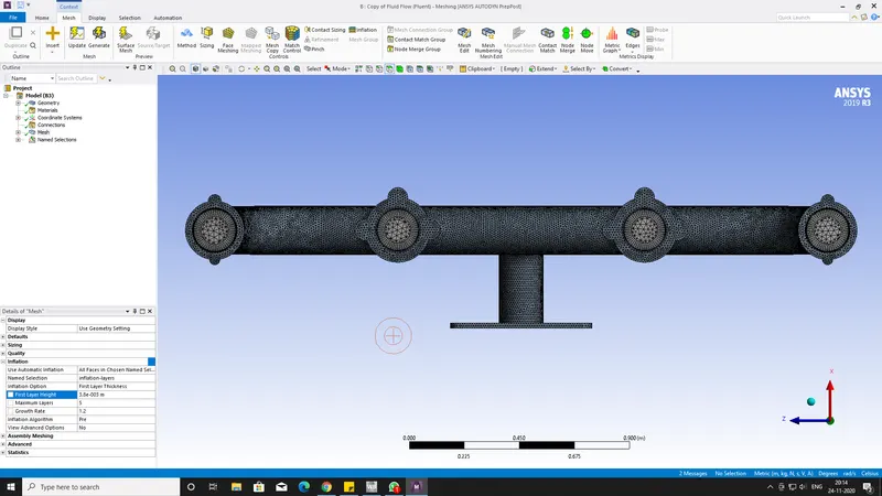
Mesh is similar for both the solver only the inflation layer "First Layer Height" changes.

K-Epsilon

K-Omega:

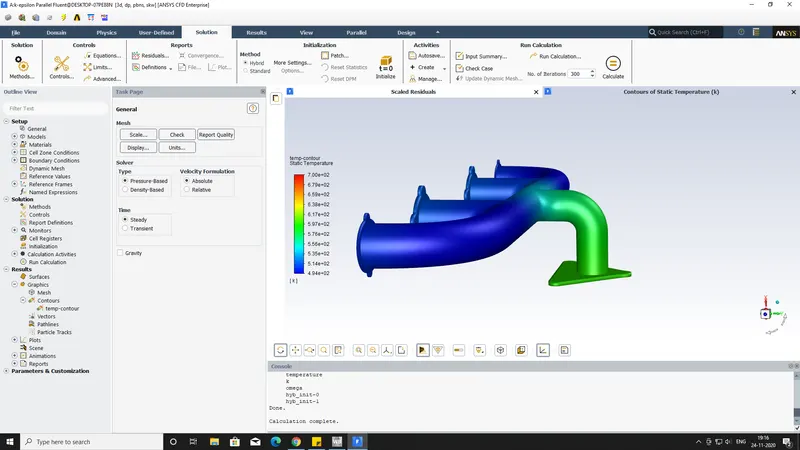
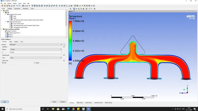
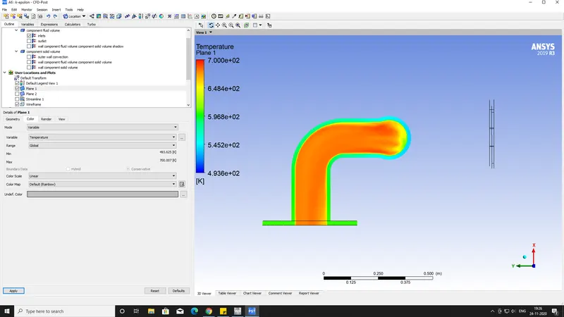
3) Heat transfer coefficient, velocity & temperature contours:

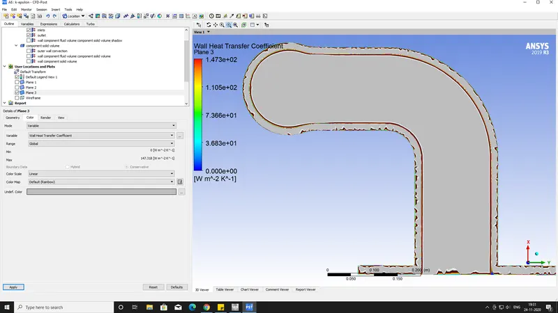
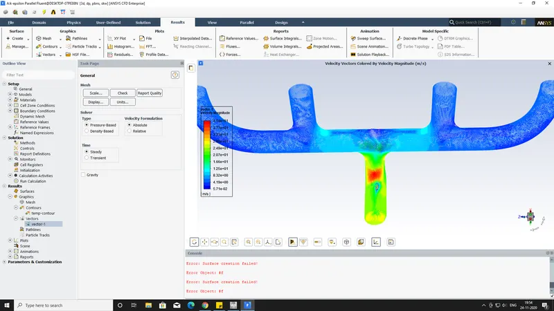
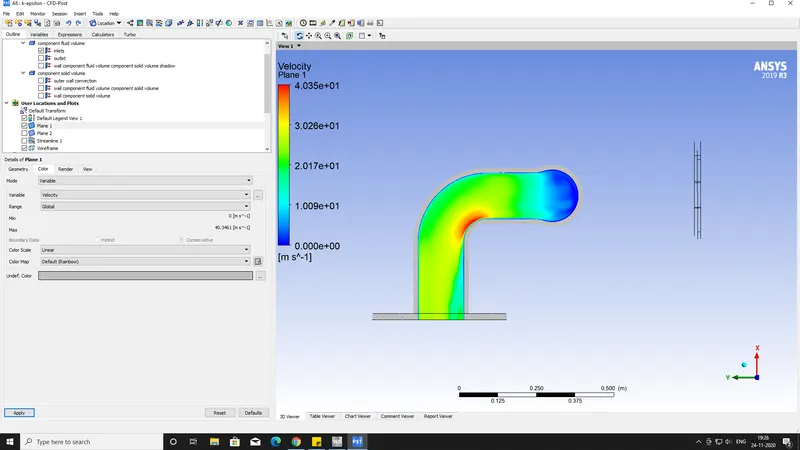
K-Epsilon Results:

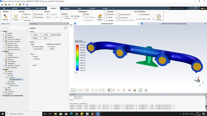
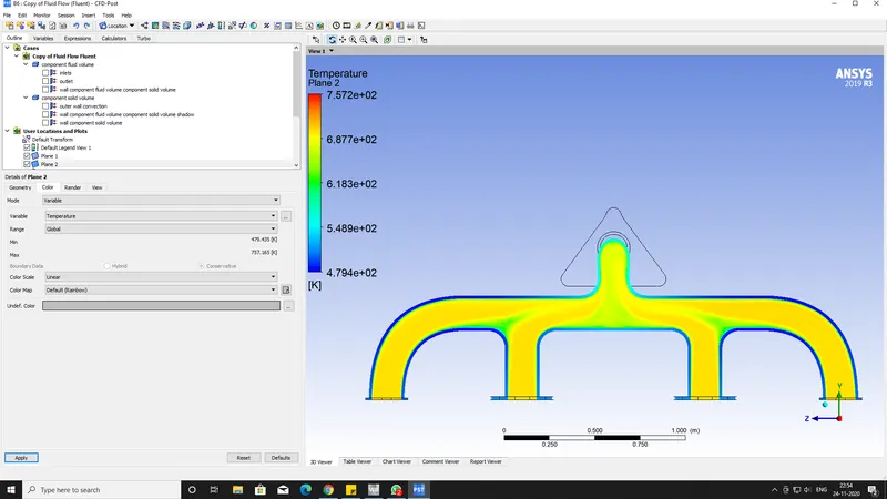
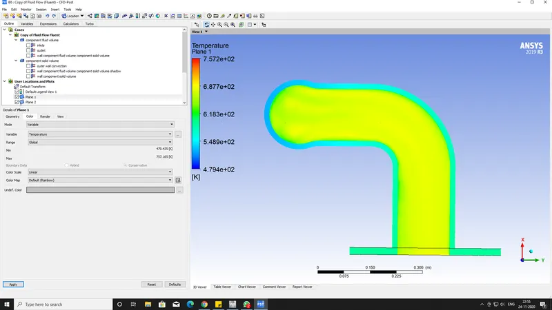
Temperature and Velocity contours:

K-Omega Results:

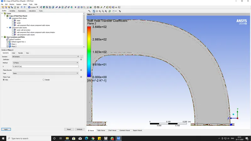
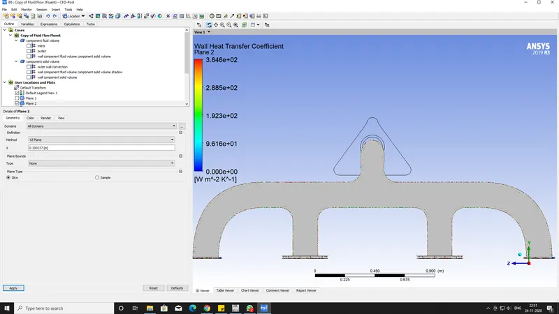
Temperature and Velocity contours:

The Wall Heat Transfer Coefficient Results:

Wall heat Transfer Coefficient	Values
K-Epsilon	147.3 `W/(m^2K)`
K-Omega	384.6 `W/(m^2K)`

4) Validating the simulation:

Heat Transfer Coefficient

`dotq = alpha*triangleT`

`alpha=Nu*(lamda_f)/(L)`

`dotq` = heat flux

`alpha=` heat transfer coefficient

`triangleT`= temperature difference between wall and fluid

`lamda_f`= thermal conductivity of the fluid

L= characteristic length of the system

Nu = Nusselt number

• There are a couple of ways to verify or to validate the results.

1. By doing the grid dependency test and comparing the end results with the analytical values.
2. Using dimensionless numbers like Reynolds, and Nusselts numbers we can validate our results. As the Reynolds number deals with the fluid flow properties and whereas, the Nusselts number deal with heat transfer coefficient.

• As said before, In principle, the Nusselt number is not a material constant but is determined to a large by the properties of the flow with regard to velocity and thermal conduction. The flow velocity is characterized by the dimensionless Reynolds number. The thermal conductivity is also taken into consideration with a dimensionless parameter, the so-called Prandtl number. The Prandtl number describes the transport of momentum between flowing fluid layers in relation to the transport of heat by thermal conduction.

`bar(Nu) = bar(Nu)(Re,Pr)`

Conclusion:

• There are a few crucial points I would like to mention here. First of all, while working in SpaceClaim make sure to enable topology to"share" and fix the errors like coinciding the solid and fluid volume inlet dimensions.
• In Meshing make sure to increase the face meshing at the inlet circle as low as possible to look like a circle rather than a polygon. Y+ calculation is the most important in this whole simulation as we are intended to find the wall heat transfer coefficient values.
• The Y+ value is not similar for both the turbulence models. K-Omega has a lower range and K-Epsilon has a higher range.
• After analyzing the results I conclude that the K-Omega turbulence model is suitable for this type of simulation.
• I don't totally disagree with the other turbulence model here the need is different and K-Omega best suits our requirement.
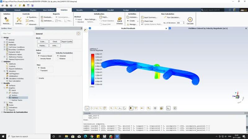
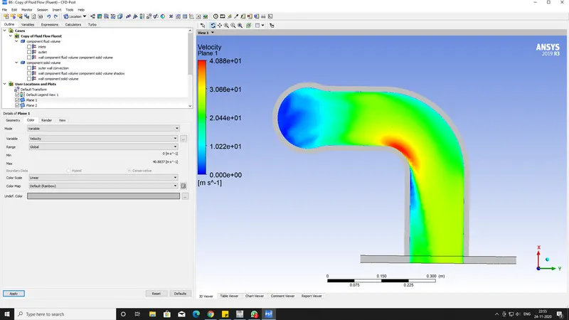
• It is very fascinating to explain the velocity profile. The velocity is maintained almost constant at all the portions of the inlet pipes but when it reaches the outlet pipe the velocity increases tremendously. As shown in the below picture.

• The red color at the bent portion represents the higher velocity. This is due to the fluid coming from all the four inlets and this makes it increase the velocity and as well as temperature too.