Rayleigh Taylor Instability Challenge

Aim: To present the Rayleigh Taylor Instability by performing the exchange of fluids through two different surfaces.

Introduction: In this analysis, we will be drawing two surfaces. Placing them one upon the other as shown in the below picture. Here we will be changing the mesh size and create a UserSpecified material and will compare the results.

1) Practical CFD Models Based on The Mathematical Analysis of Rayleigh Taylor Waves.

• K-L Turbulence model for Rayleigh Taylor and Richtmyer-Meshkov instabilities: K-epsilon turbulence model is the most common model used in computational fluid dynamics to simulate mean flow characteristics for turbulent flow conditions. It is a two equation model that gives a general description of turbulence by means of two transport equations (PDE's).
• Potential flow models of Rayleigh Taylor and Richtmyer Meshkov for bubble fronts: A potential flow model of Rayleigh Taylor and Richtmyer Meshkov bubbles on an interface between an incompressible fluid and a constant supporting pressure (Atwood Number = 1) is presented. Competition, for both the Rayleigh-Taylor and the Richtmyer-Meshkov instabilities.
• Kelvin-Helmholtz/Rayleigh Taylor Hybrid Model: This is particularly used for modeling spray atomization, an Example of fuel spray in diesel engines. 
• Rayleigh-Taylor Instability with two-fluid model and interface sharpening: The free surface flows are successfully modeled with one of the existing free surface models, such as = level set mothed, volume fluid method, front tracking method, two-fluid model (two momentum equation) with modified interphase force and some others.
• Discrete Boltzmann Model(DBM): Here in DBM it is used to simulate the multi-mode Rayleigh Taylor instability in a compressible flow. This DBM is physically equivalent to a Navier-Stokes model supplemented by a coarse-grained model for thermodynamic non-equilibrium behavior.

2) MESH DEPENDENCY TEST: Before going to the meshing, the below picture depicts the geometry of the model. We have created two blocks one upon the other and their topology is set to "SHARE".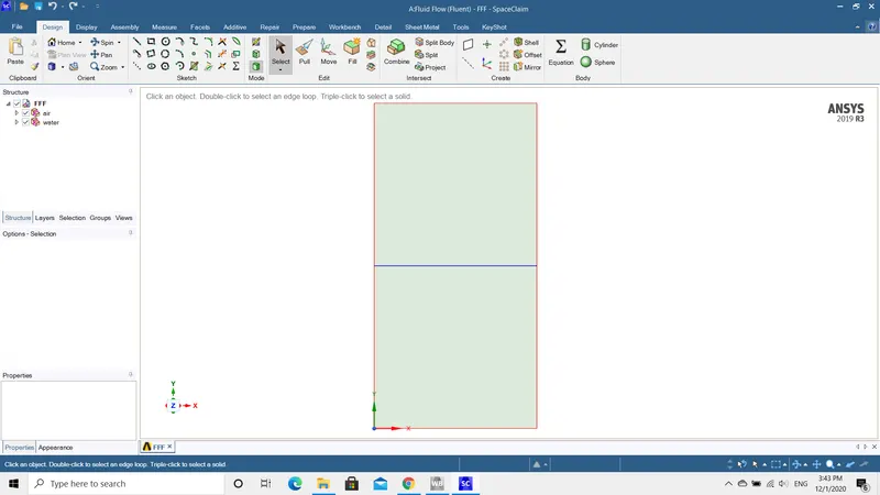

• According to the given description, the simulation should be carried on two types of mesh size.
• First, the base size is 0.5.  

 

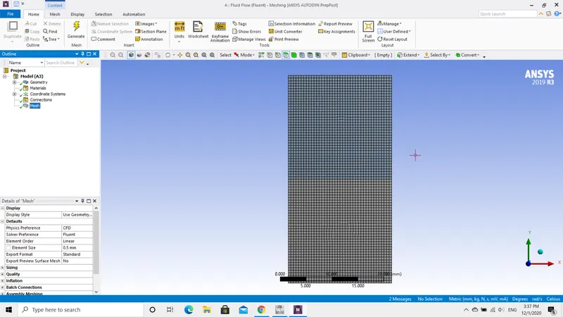
• Moving to the fluent, as per our requirement we need two materials and the air is the default material.
• Water material should be added. There are a couple of things to be enabled.
• The type of method here we used is the Transient method and hybrid initialization.
• The multiphase option should be enabled. After that, enable the hybrid initialization and set the patch, and run the calculation but setting an appropriate time step.
• The below animation represents the mesh size of 0.5 and default water properties.

• REFINING THE MESH SIZE: For the next simulation I have reduced the mesh size to 0.09. All the other settings which I have explained above are similar here and the same materials.

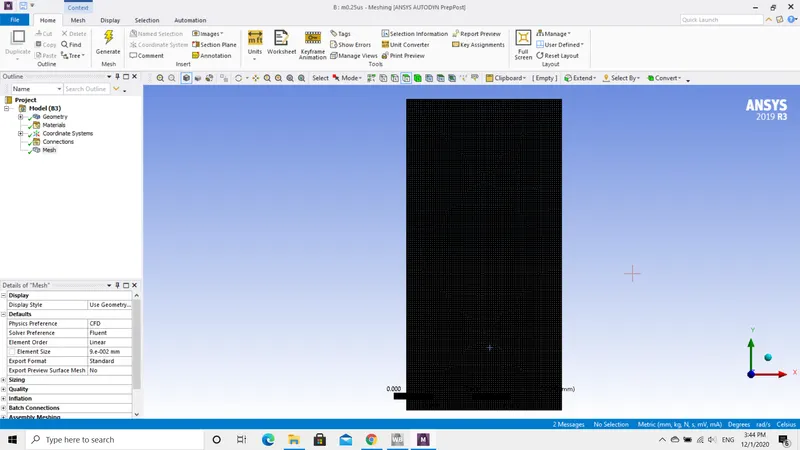
• The below animation video represents the refined mesh but with different water properties.
• The density of the water is 400 kg/m^3 and viscosity is 0.001 kg/m-s.

• WHY STEADY-STATE APPROACH MIGHT NOT BE SUITABLE FOR THIS TYPES OF SIMULATION: In this type of simulation cannot use a steady-state solver this is due to the following reason.
• First of all, the analysis which we are performing here is time dependent and the steady-state solver is not time dependent and hence we may not be able to see the instabilities during the mixing of water and air.
• So, whenever there is a simulation that is dependent on time only Transient Simulation is suitable.

ATWOOD NUMBER: The Atwood Number is a dimensionless number in the fluid dynamics used for the study of hydrodynamic instability in density stratified flows. 

• It is a dimensionless density ratio defined as the density of heavier fluid=density of the lighter fluid.
• In this challenge, we ran two cases one with default water properties and the other with different water properties.

case 1:

`A= (rho_1-rho_2)/(rho_1+rho_2)`

`rho_1=997`

`rho_2=1.225`

A=`(997-1.225)/(997+1.225)`

A=`0.997545`

case 2:

`A= (rho_1-rho_2)/(rho_1+rho_2)`

`rho_1=400`

`rho_2=1.225`

A =`(400-1.225)/(400+1.225)`

A =`0.993893`

In both cases, the Atwood number is approximately close to one. This means the lighter fluid is at the bottom and forms bubbles while moving up. This proves that our results or simulation is valid.

CONCLUSION:

• I would like to conclude that, I have Performed the simulation by changing the mesh element size. As it is well known the smaller the mesh size smoother the simulation. 
• I have also changed the material properties as mentioned in the question and uploaded the animation above.
• I calculated the simulation about 1000 time steps and the results turn to be converged.
• In the next simulation, I could able to achieve the mesh element size to 0.25mm.
• After comparing both the simulation i.e, with default water properties and on the other hand with user-defined material property, it is clear that fluid with higher density settles faster than the fluid with lower density.
• I have attached all the documents, pictures, and animation videos below.