Mixing efficiency
MIXING EFFICIENCY
- In this challenge, we are analyzing flow through a T shaped pipe. Where the temperature through the Inlet at x-direction is greater than the temperature at the inlet y-direction.
- In the next step, we change the inlet velocity. The hot inlet velocity is 3 m/s which is standard and the cold inlet(Y-direction) has a momentum ratio of 2,4.
- In this analysis, we perform the test on two different geometries. one is a short pipe length and another is a long pipe length and plot the differences.
- Each geometrical structure undergoes two types of flow conditions i.e, k-epsilon and k-omega.
- Above mentioned points are executed in the Ansys student version software and related screenshots and documents are attached below.
MIXING-T (Short Length): Geometry:
- First, we create a fluid flow standalone in the workbench environment, and next, we can either create new geometry in the SpaceClaim or we can directly import the geometry into the SpaceClaim.
- In my case, I have imported the geometry for all the processes and extracted the volume as shown below.
- After extracting "suppress the solid body for physics". As we are intended to study only the fluid flow.
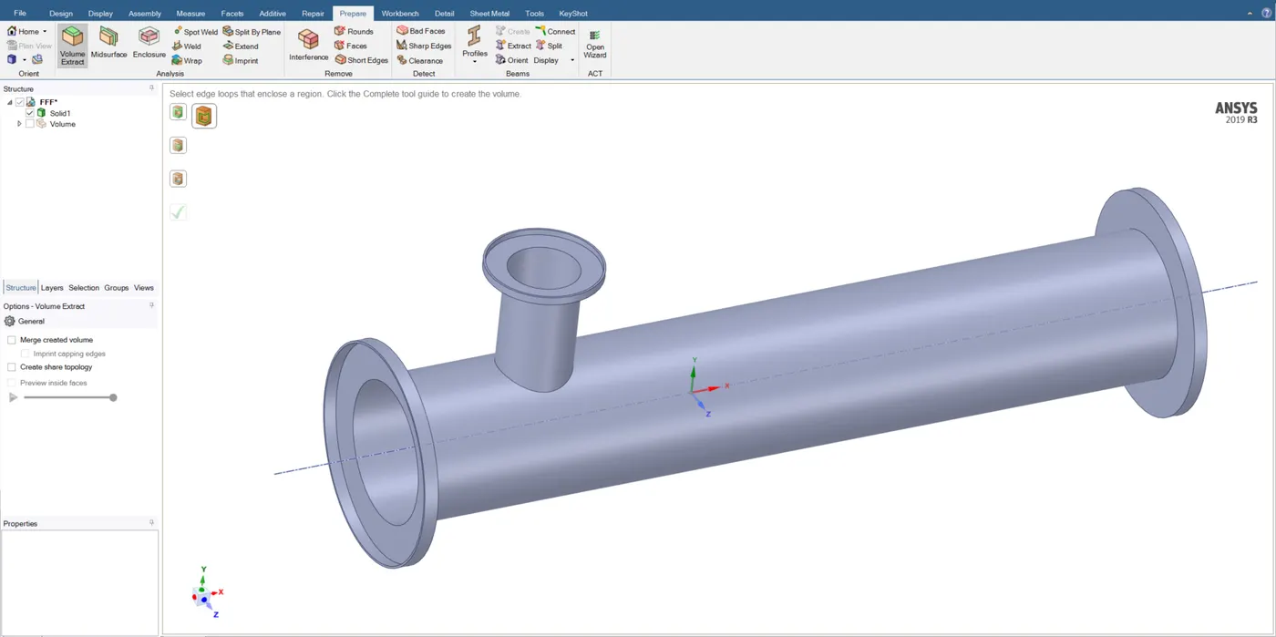
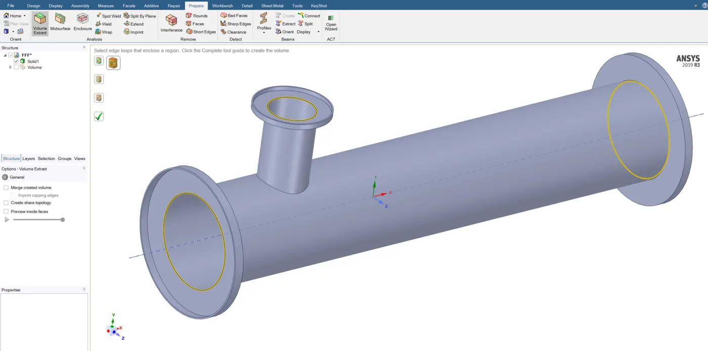
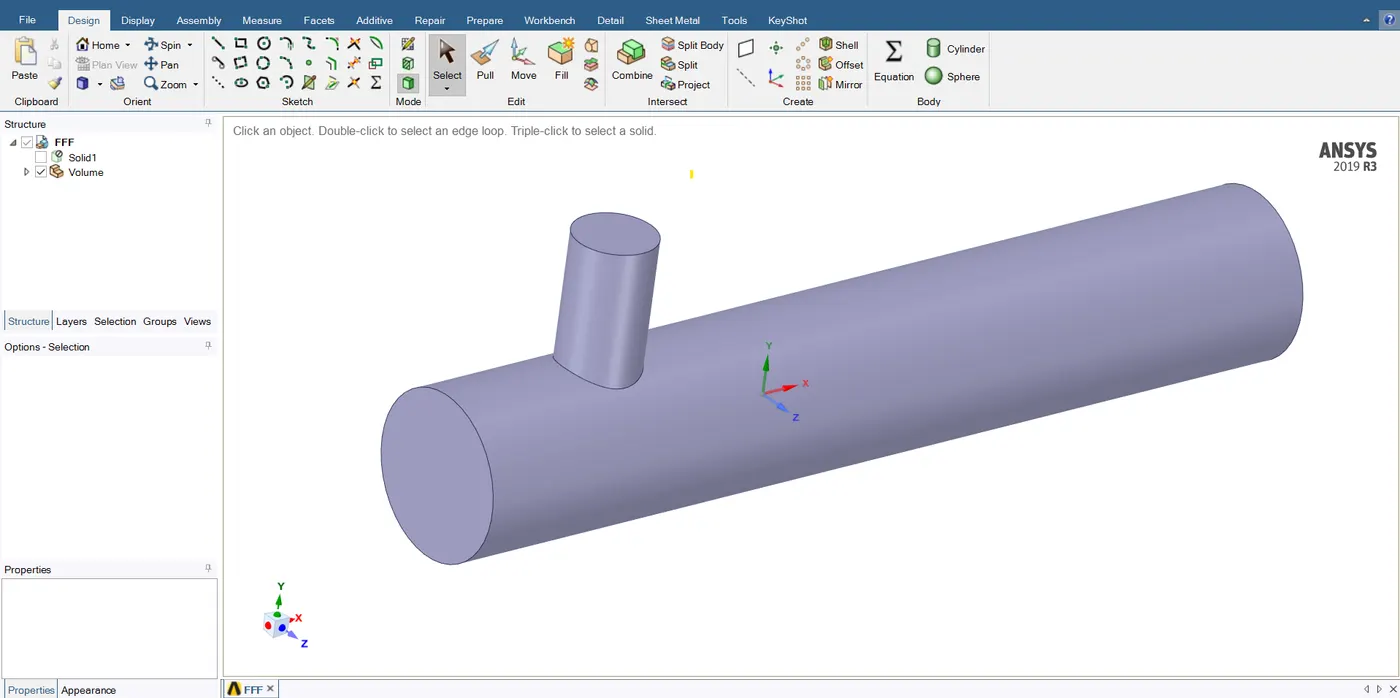
- After importing the geometry I have extracted the volume using the edge selection method and suppressed the solid for physics.
- The above pictures are the results.
Meshing:
- Close the SpaceClaim and open the meshing window. Set the meshing size, name the faces of the geometry and generate the mesh.
- By defining the boundaries or faces of the geometry helps in postprocessing th fluent.
- I have set the mesh sizing to 2e-3 (0.002).
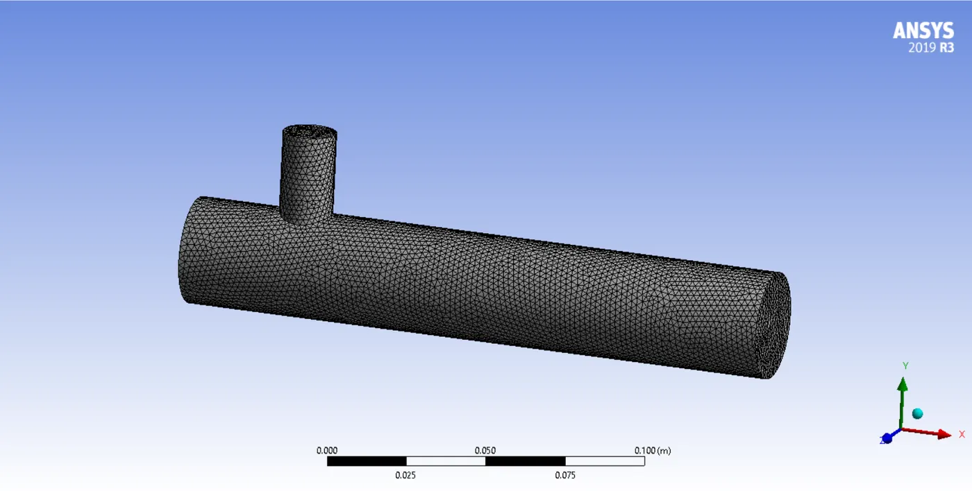
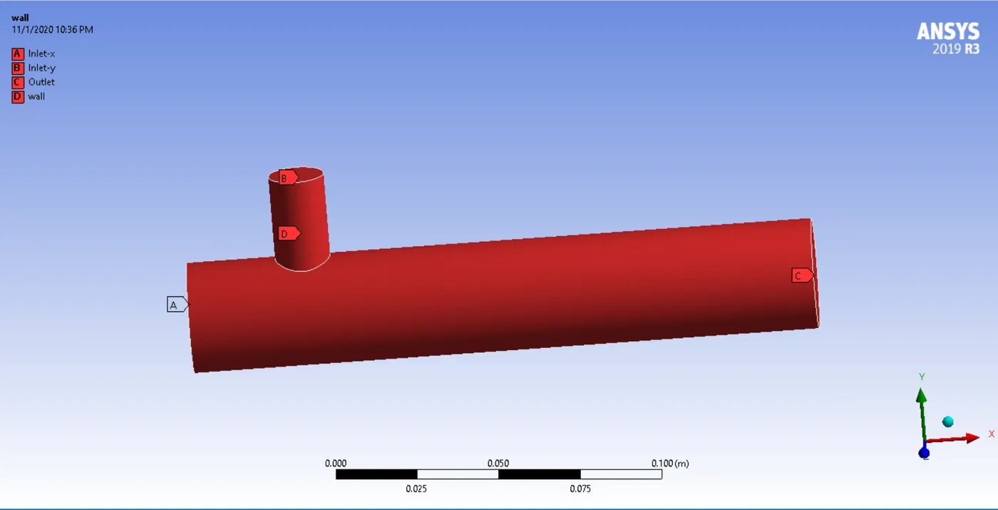
- The above two pictures depict the mesh sizing and labels of the boundaries and faces.
Fluent Setup:
- Before opening the fluent do the setup for fluent. Select the double precession option and set the number of processors you wish to allot.
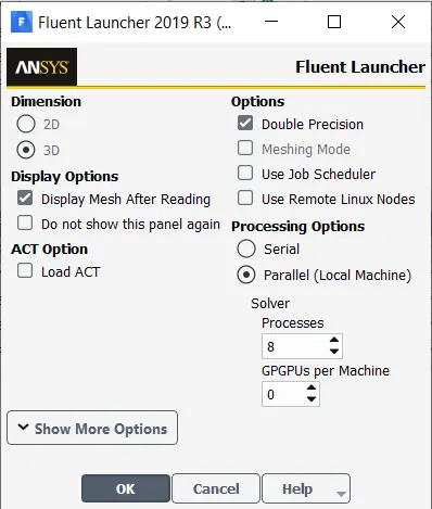
- Before editing the fluent there are a couple of changes to be made in the standalone setup.
- choose double precision and parallel processing.
Fluent settings:
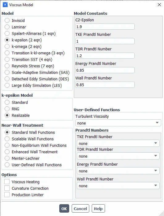
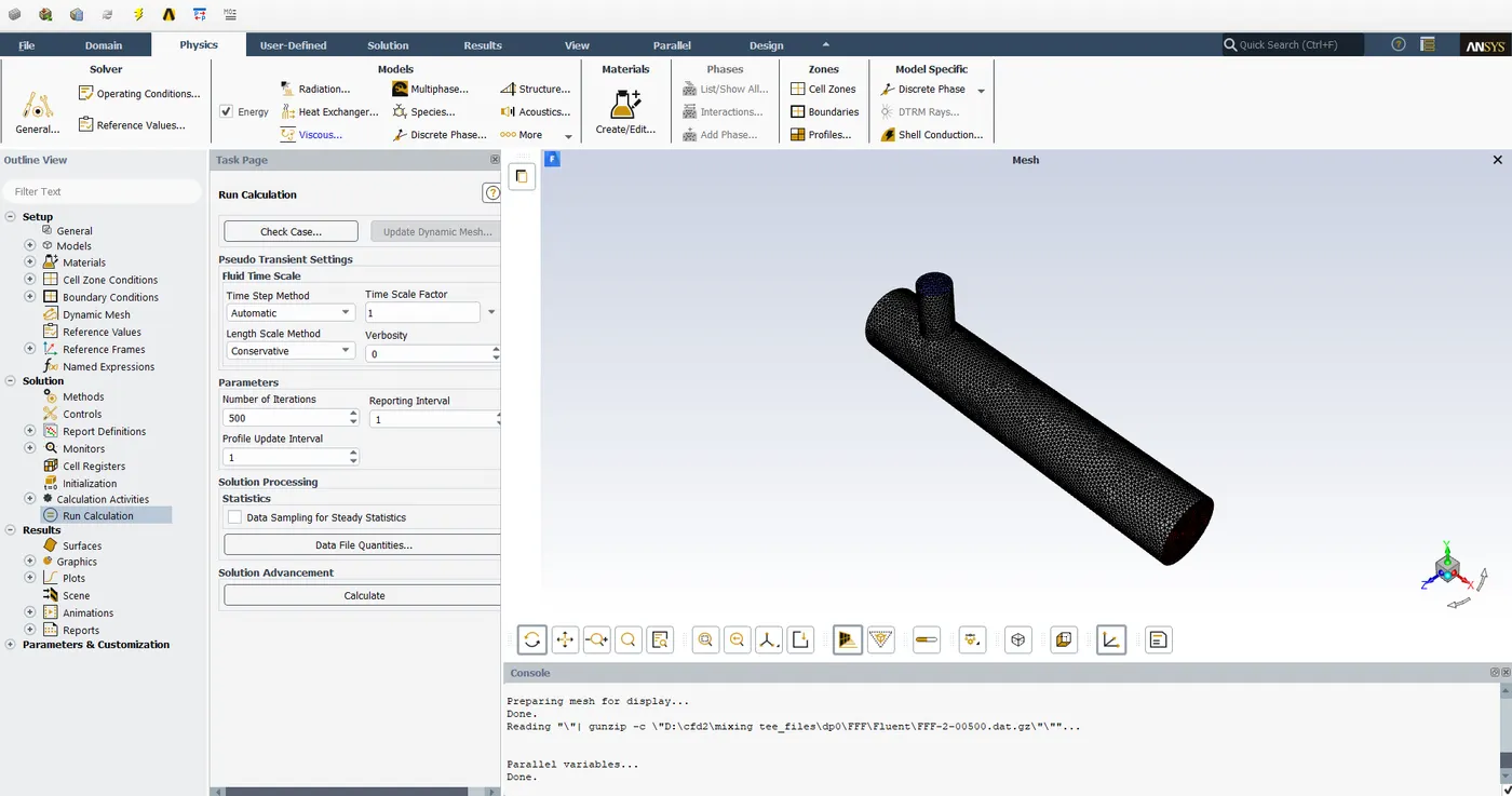
- First, we have to check the meshing quality.
- As we are performing temperature exchange to select the energy option. As shown in the second picture.
- There are some operations to perform after this.
- Go to -> physics-> cell Zones-> check the type of fluid.
- Go to -> physics-> Boundaries-> edit Inlet-x -> change velocity to 3 m/s and the temperature to 36 degree centigrades.
- Similarly, select Inlet-y to change the velocity to 6 m/s for the first case and 12 m/s in the second case but the temperature remains the same at 19-degree centigrades.
- I am plotting two graphs, we can say monitoring different types of results at the outlet.\
- One is Area Weighted Average and another is Standard Deviation of temperature at outlet.
- After making all the above changes go-to the solution tab and initiate an initialization and run the calculations.
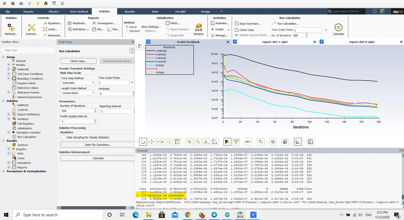
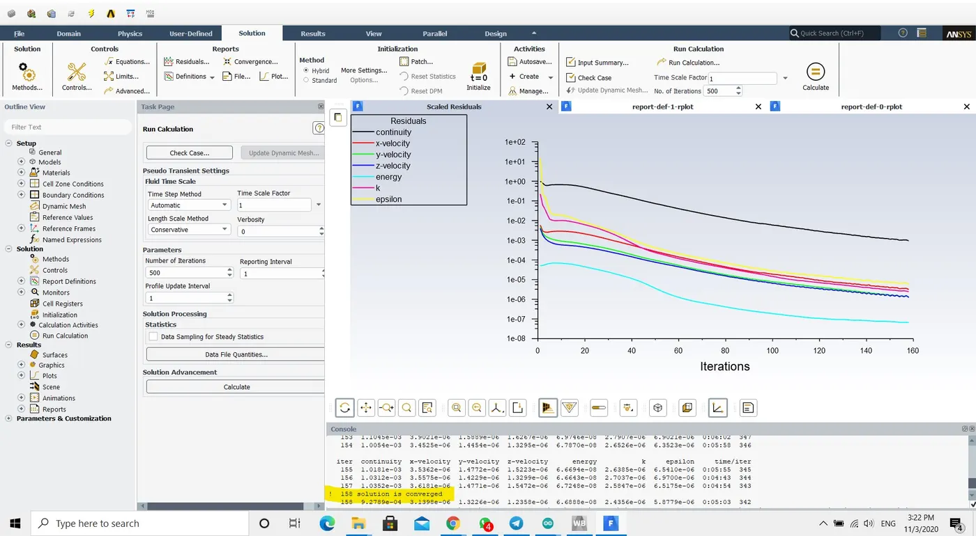
- We can run the calculations until the solution gets converged.
- Sometimes we do not receive a solution converged message, instead, we can see the scaled residual plots to be stable after a certain number of iterations.
Results:
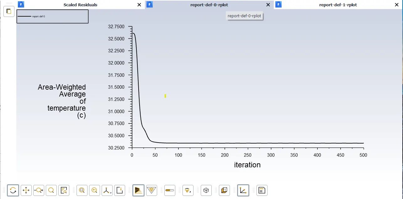
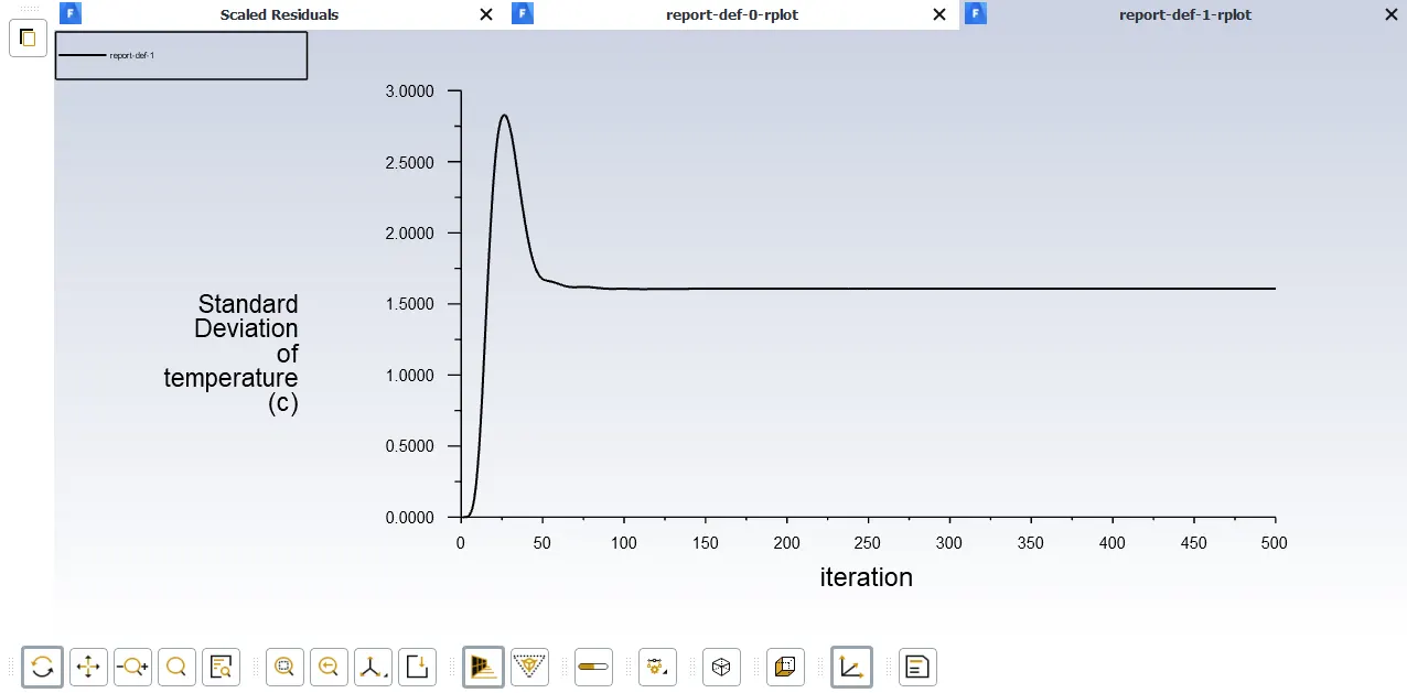
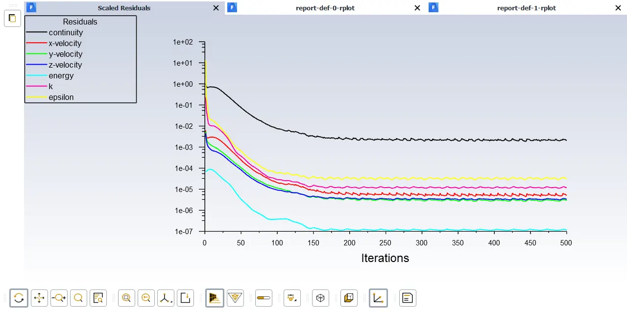
- The above plots are the results and Ansys Fluent by default plots the scaled residuals.
- In certain situations the fluent might not converge the solution in those circumstances we can analyze the above graphs and we can end the calculations if the lines are stable and steady.
- In my case, I faced the above problem but with 200 Iterations my solution is stable and I presumed that it is converged.
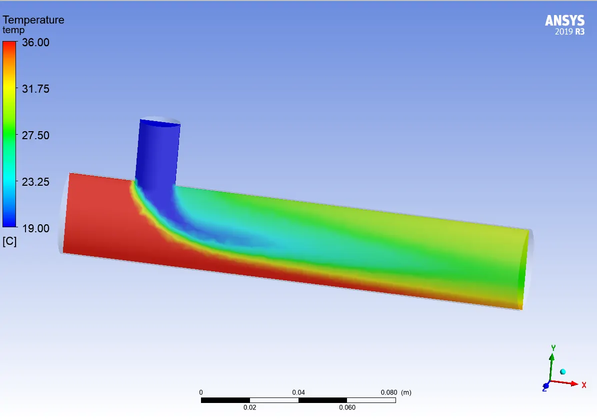
- After performing the calculations we proceed with the postprocessing window. There we can execute the velocity and temperature plot in graphical representations.
- Below are the graphical representations from the CFX.
Temperature:
Velocity:
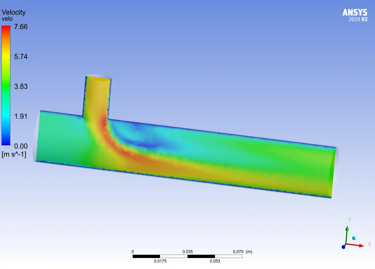
In the above profiles, the colors define the values of the elements we are looking for.
-----------------------------------------------------------------------------------------------------------------------------------------------------------------------------------------------------------------------------------------------------
- According to the given instructions in the challenge, we have to perform two different flows, two different inlet velocity in the y-direction, and these conditions are applied to the two different geometries.
- In the above simulation, I have applied K-epsilon flow and inlet velocity in the y-direction is 6m/s and the type of geometry is a short pipe.
- In further steps, I will present the other cases.
- For the rest of the process, geometry and mesh are similar so In order to build the standalone from the scratch, I have linked one standalone to another as shown in the below picture.
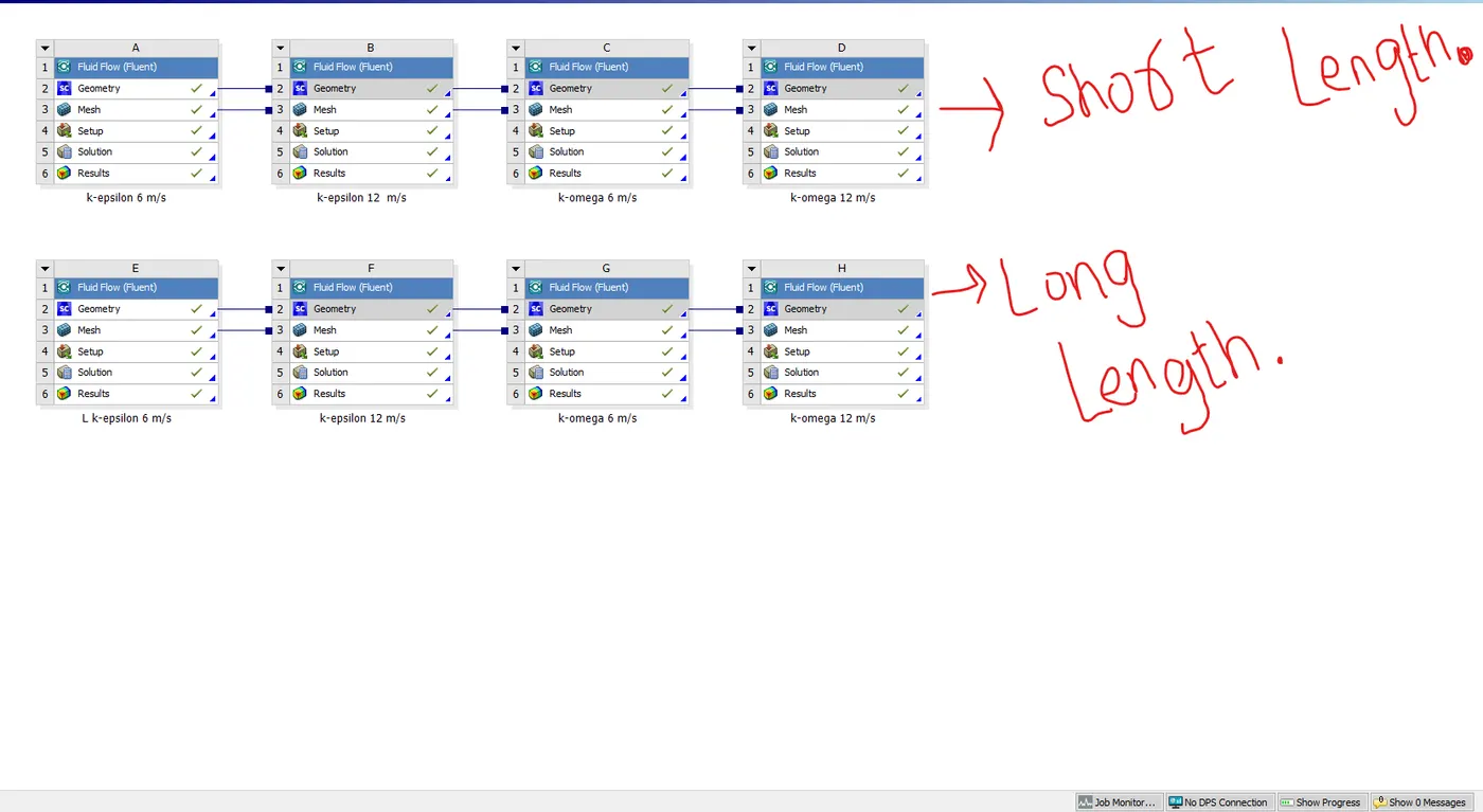
- The standalone A, B, C, D represents the Short Length Geometry and whereas, E, F, G, H represents the Long Length Geometry.
- I have renamed all to the standalone to identify the type of flow.
- by doing this we can save a good amount of time.
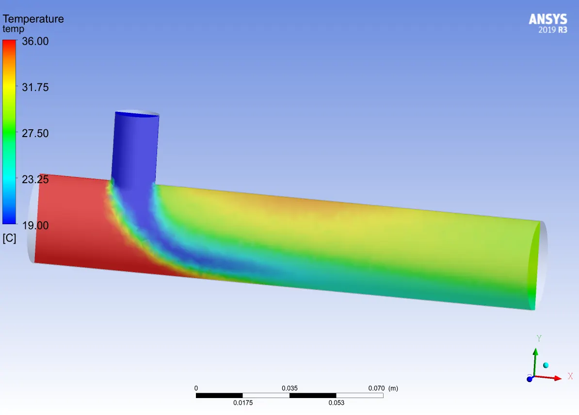
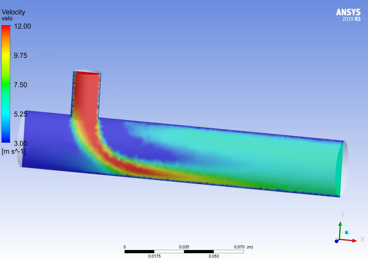
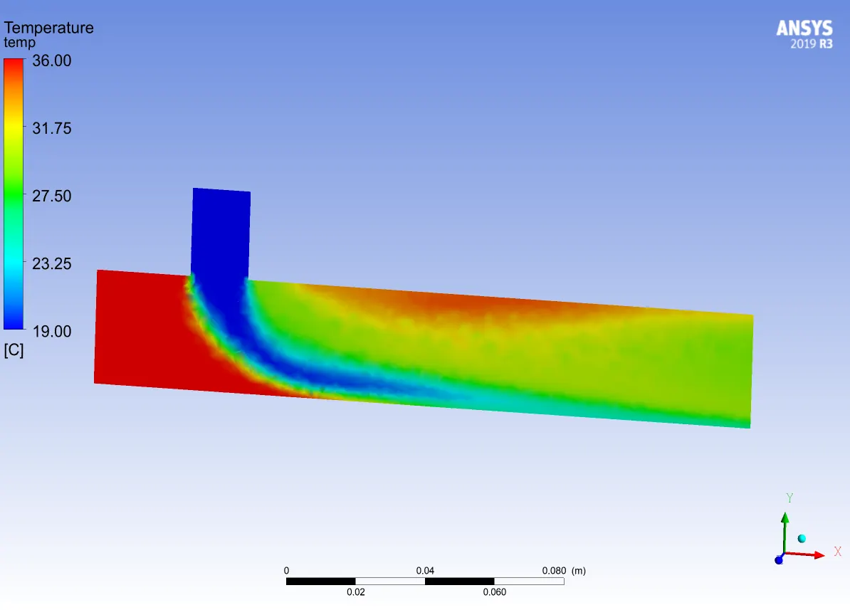
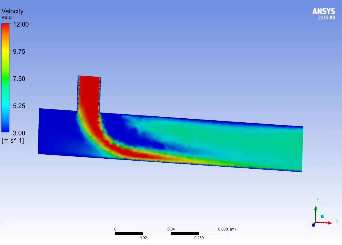
THE FOLLOWING PICTURES REPRESENTS THE CFX RESULTS OF THE ANALYSIS:
Geometry = Short Pipe
Type of flow = k-epsilon
Velocity = 12 m/s
*Temperature Profile: *Velocity Profile:
Converged Plottings:
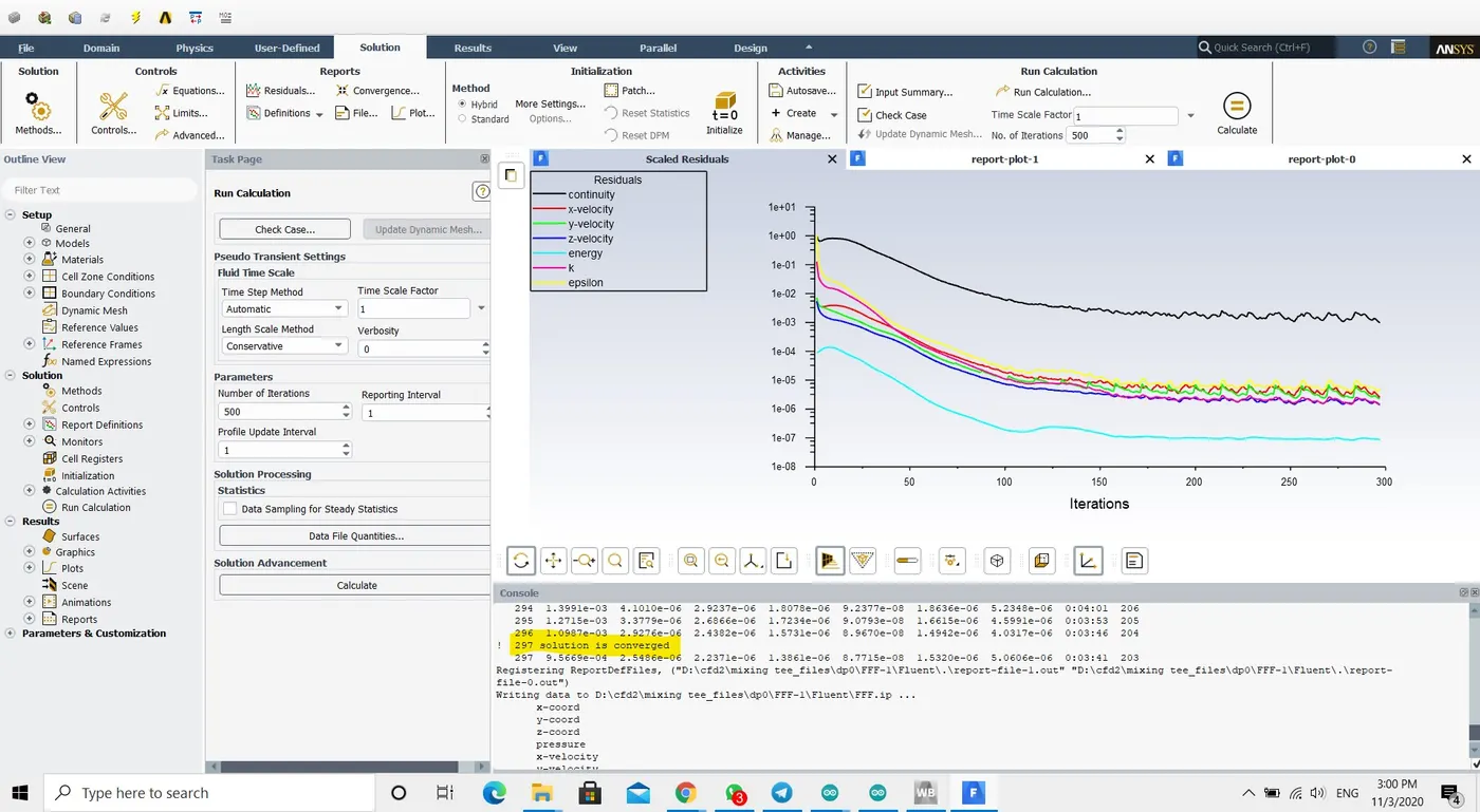
Geometry = Short Pipe
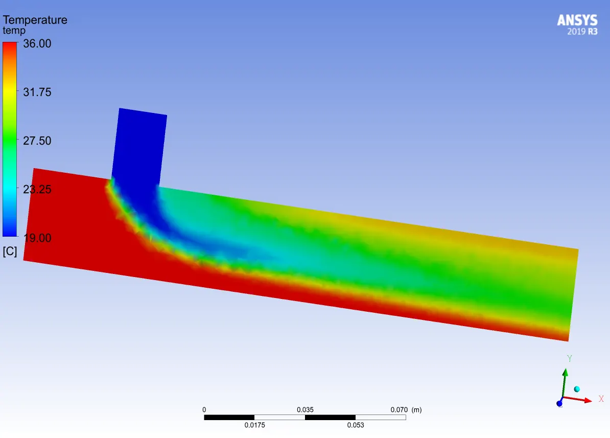
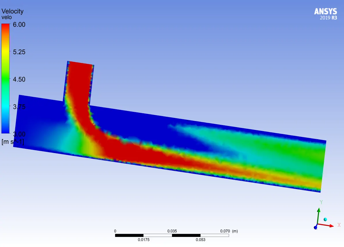
Type of flow = k-omega
Velocity = 6 m/s
*Temperature Profile: *Velocity Profile:
Converged Plottings:
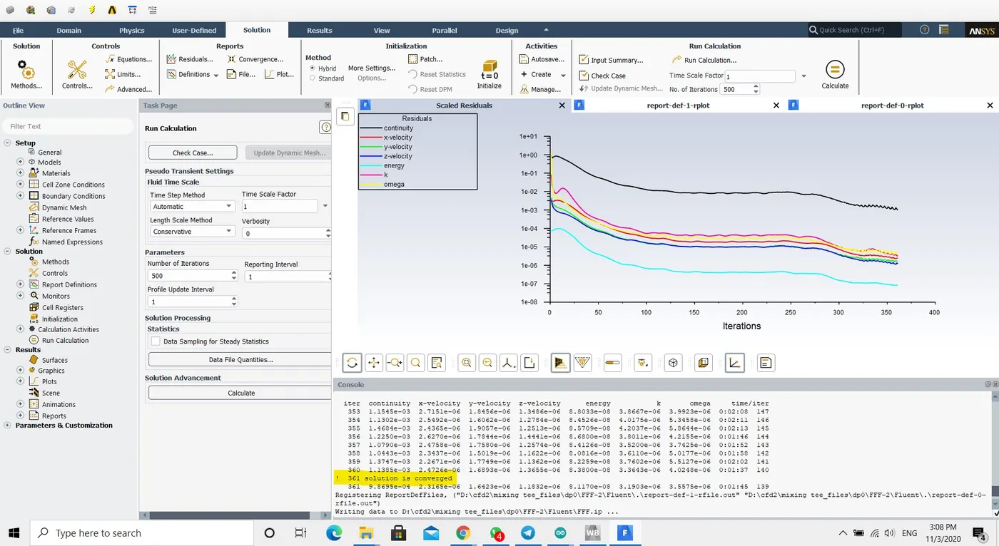
Geometry = Short Pipe
Type of flow = k-omega
Velocity = 12 m/s
*Temperature Profile: *Velocity Profile:
Converged Plottings:
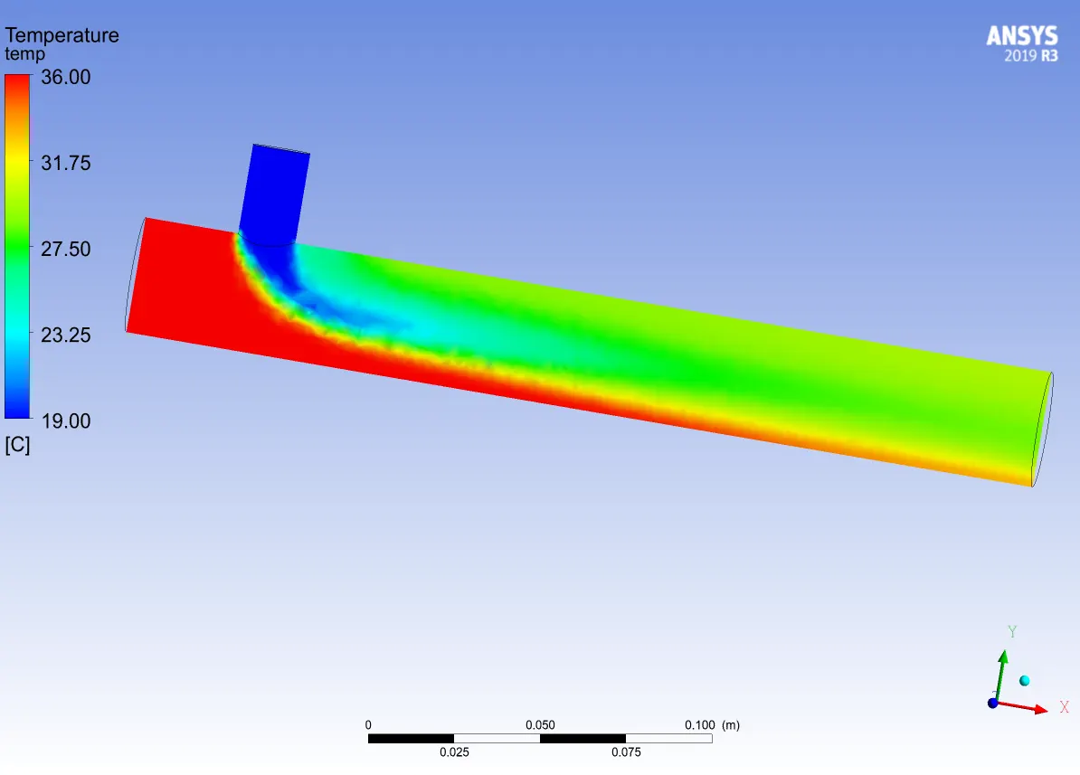
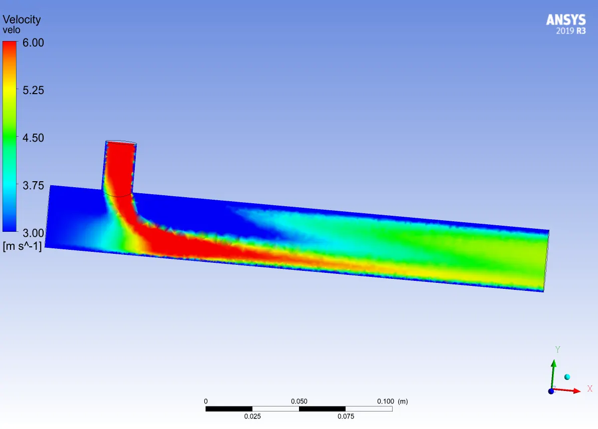
Geometry = Long Pipe
Type of flow = k-epsilon
Velocity = 6 m/s
*Temperature Profile: *Velocity Profile:
Converged Plottings:
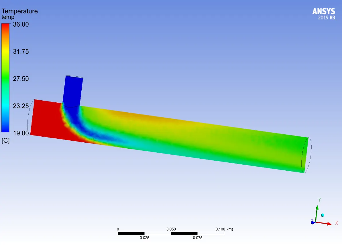
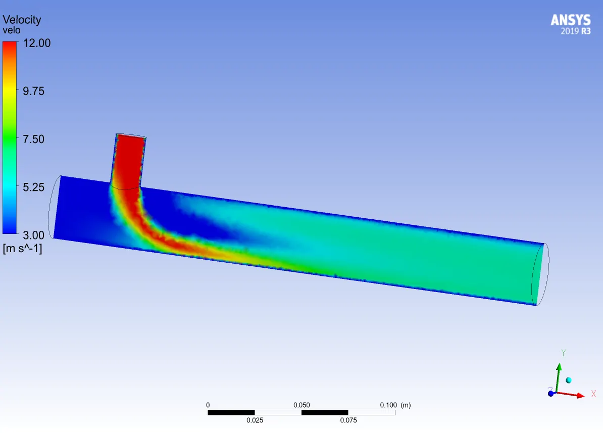
Geometry = Long Pipe
Type of flow = k-epsilon
Velocity = 12 m/s
*Temperature Profile: *Velocity Profile:
Converged Plottings:
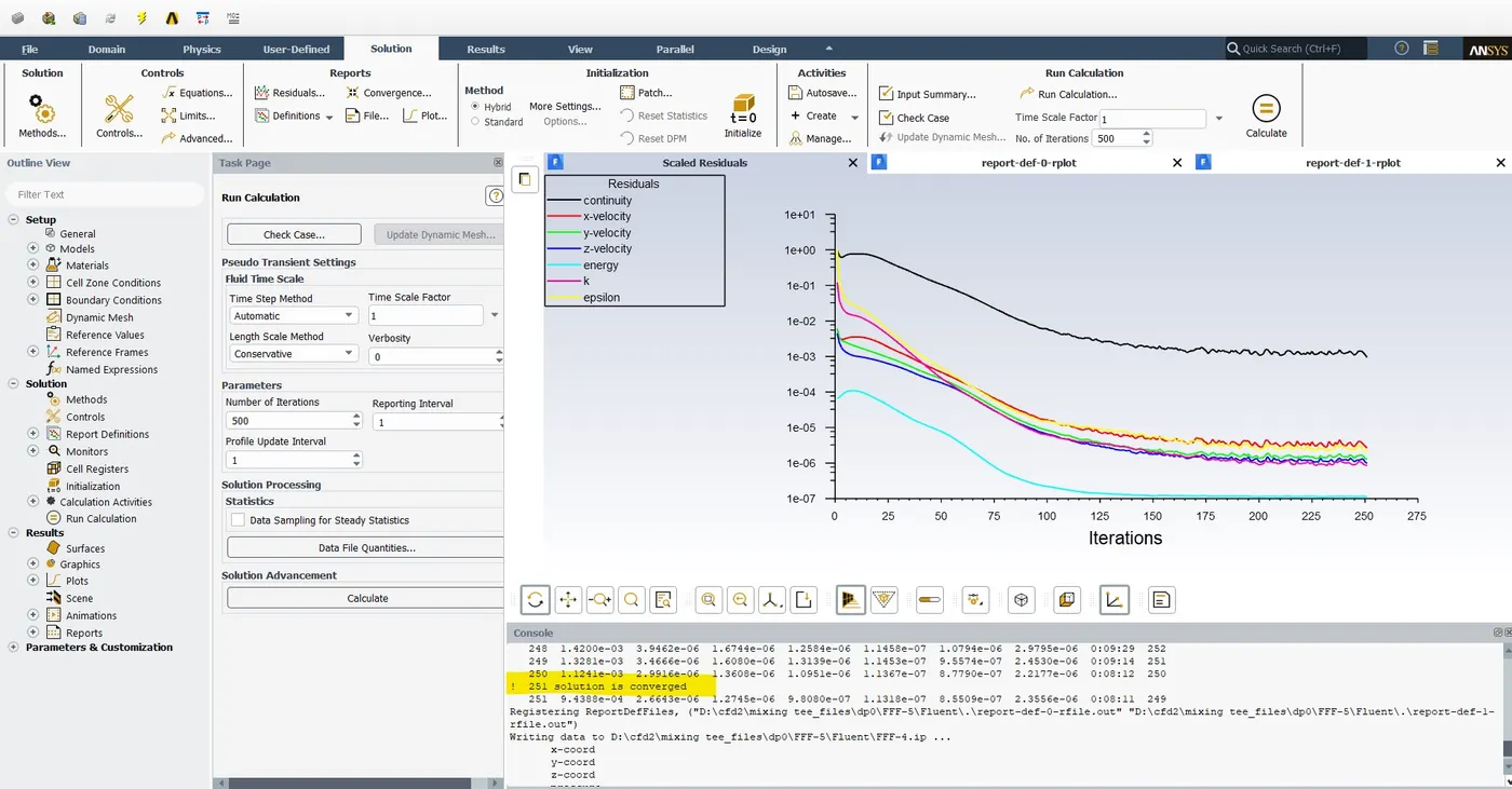
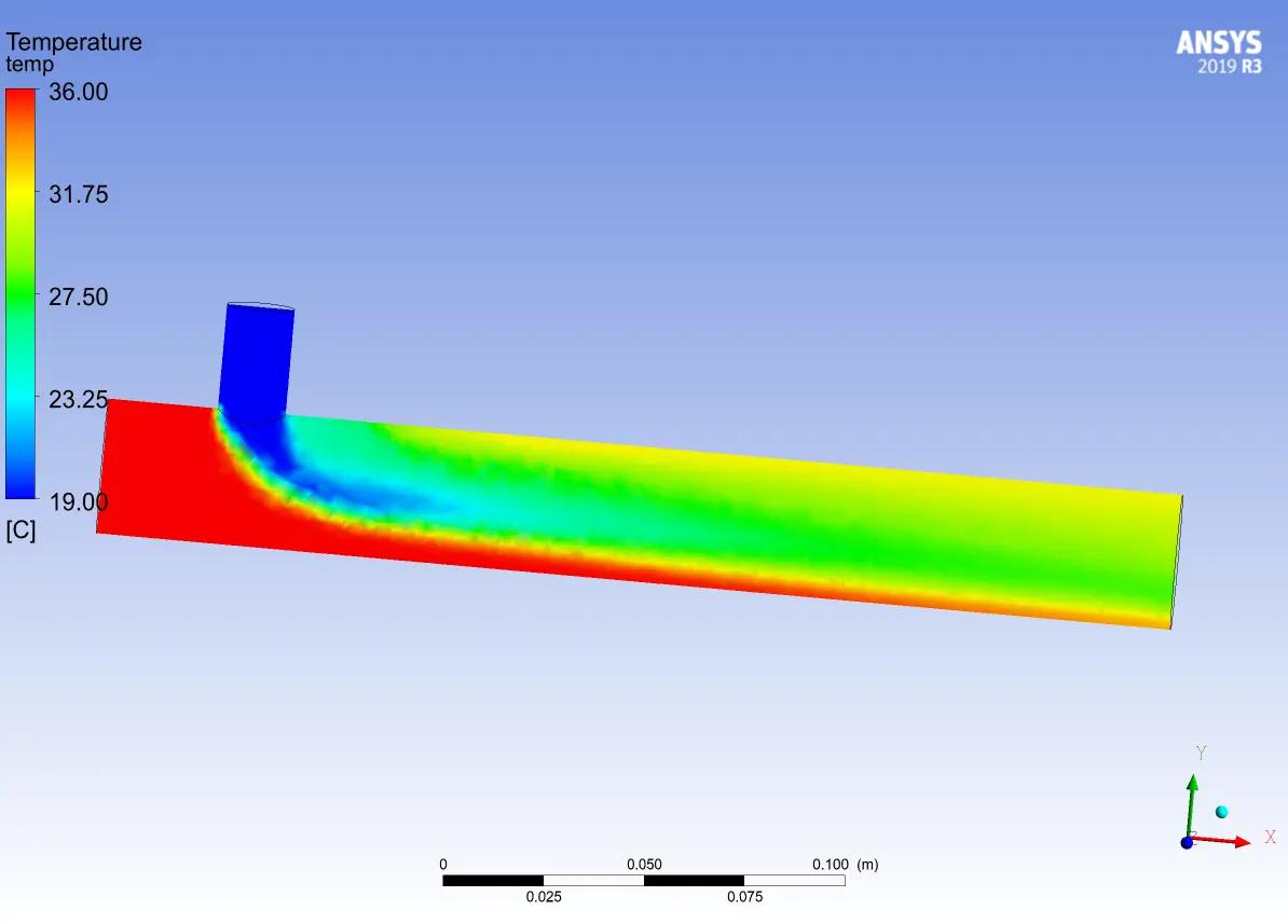
Geometry = Long Pipe
Type of flow = k-omega
Velocity = 6 m/s
*Temperature Profile: *Velocity Profile:
Converged Plottings:
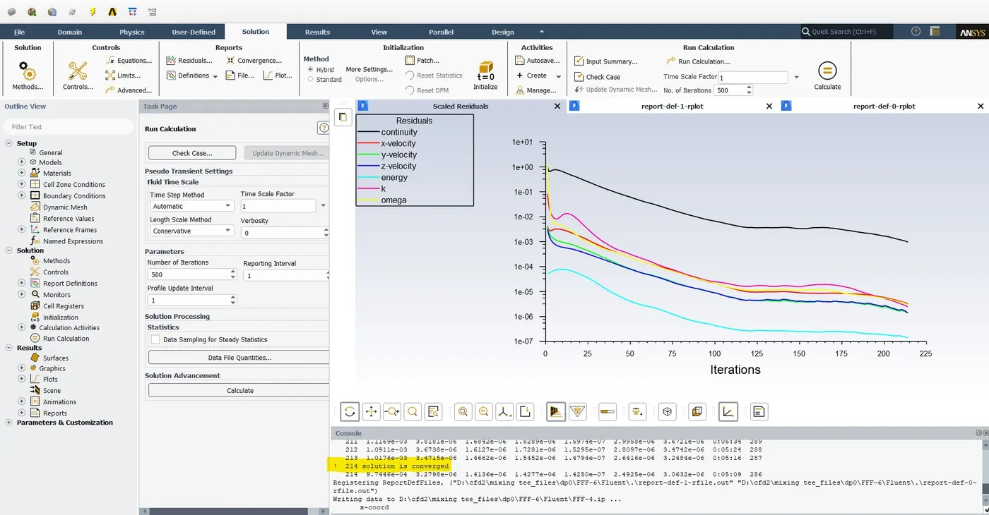
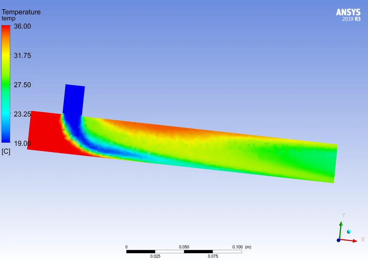
Geometry = Long Pipe
Type of flow = k-omega
Velocity = 12 m/s
*Temperature Profile: *Velocity Profile:
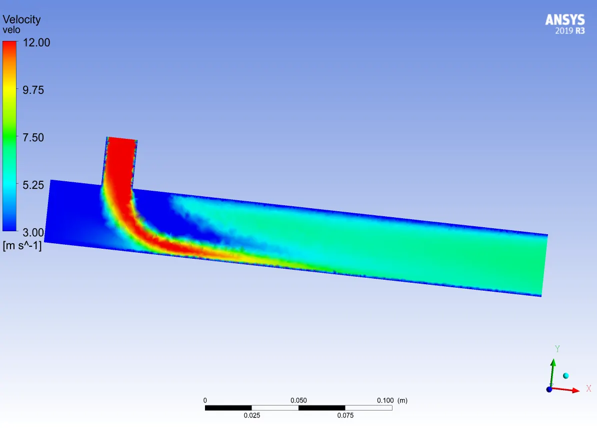
Converged Plottings:
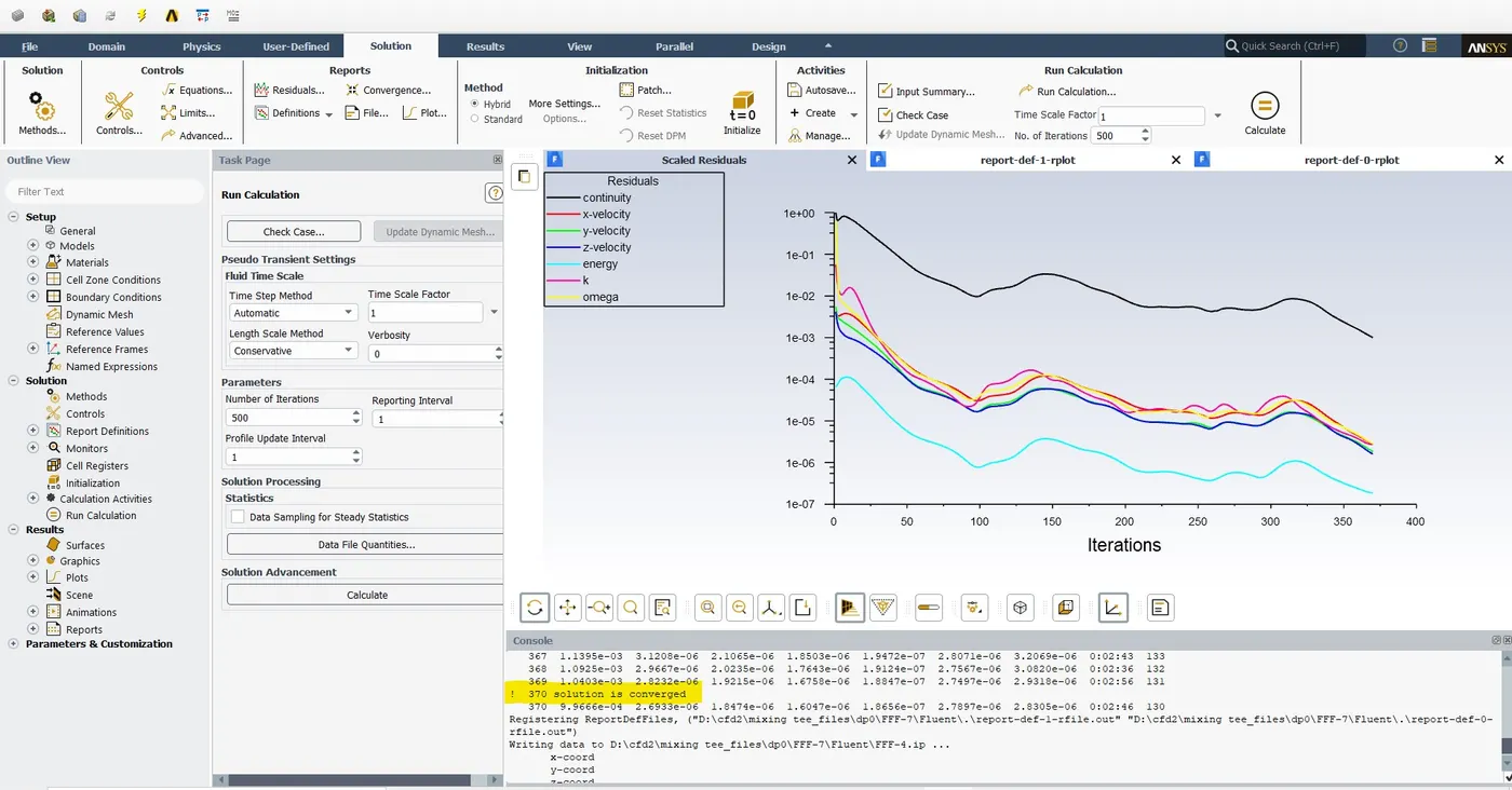
Mesh Independent Test:
*Mesh Size 0.002:
0.003 Mesh Size:
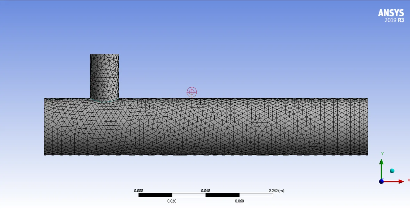
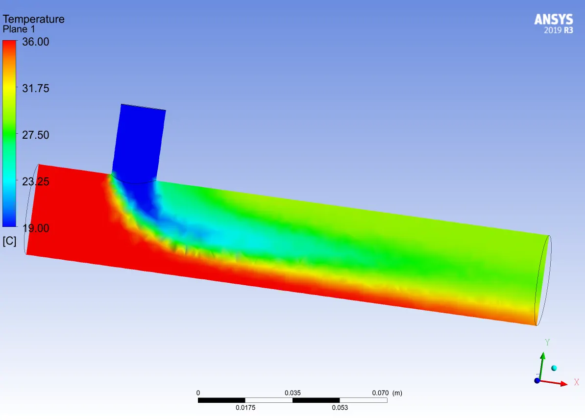
0.004 Mesh Size:
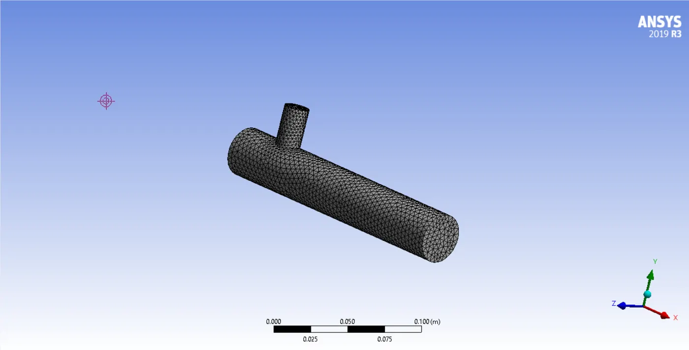
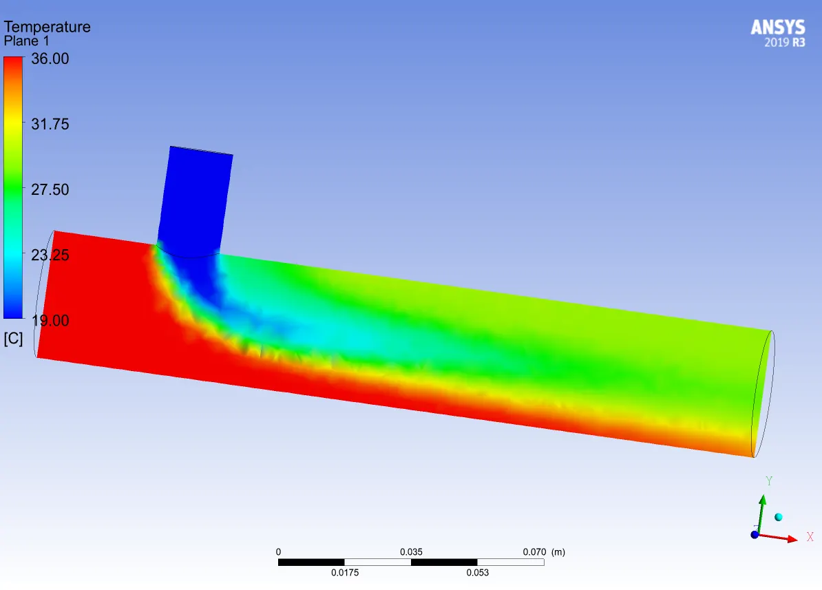
- The above pictures show the mesh sizing and the temperature profiles of the respective mesh.
- For this independent test, I have chosen the short pipe with element sizing of 2e-3, 3e-3, 4e-3 meters.
- We can clearly observe the differences between the different element sizing.
- The higher the element size the greater the values of a particular solution it might be Temperature or velocity. Depending on the simulation we are carrying.
- In our case, we are checking the temperature across the pipe and we have plotted those values on a plane.
- In the first mesh where the size is 0.002 meters the air inlet through y-direction which is represented in blue color has a longer length. Whereas, in the other size the blue color is smaller this is due to the sizing we have given.
- I conclude that the element sizing plays a major role in analyzing the geometry.
The Effect of Length and Momentum Ratio:
*Short Length, Inlet velocity in the y-direction is 6 m/s.
*Short Length, Inlet velocity in the y-direction is 12 m/s.
*Long Length, Inlet velocity in the y-direction is 6 m/s.
*Long Length, Inlet velocity in the y-direction is 12 m/s.
- First of all, for any mixing tee simulation, the average outlet temperature value depends on the velocity of the inlet temperature in normal to another flow.
- We can look at the above pictures I have mentioned the inlet velocity of the air in the y-direction (19C) with a momentum ratio of 2 and 4.
- The velocity in the x-direction is standard at 3 m/s.
- The greater the inlet velocity (y-direction) lesser than time to reduce the temperature.
- Both the length and moment ratio plays a crucial role in converging and reducing the outlet temperature.
- The longer the pipe the lesser the convergence iteration number.
I have pasted the google drive link which has the ansys workbench files of the above simulation
https://drive.google.com/drive/folders/1k3__f-9PW9SZIcjoUcQGfvgwpMx8ox9K?usp=sharing