Week 7 - Simulation of a 1D Super-sonic nozzle flow simulation using Macormack Method

Numerical Solutions of Quasi- One-Dimensional Nozzle Flows Through a Convergent-Divergent Nozzle.

Initially, every numerical solution of the flow will use any particular CFD solution.

In the intermediate steps after selecting a specific solution for the numerical equation of the flow problem. The integral form of the equations will be applied to the problems.

In the final stage, we plot the graphs of the numerical solution. These graphs represent the residual values, density, temperature, velocity, and pressure.

Physical description of the problem: Here we consider a steady-state isentropic flow through a convergent-divergent nozzle. The convergent side is connected to the reservoir and the flow enters from here and the divergent is the nozzle exit.

The pressure, temperature, density, velocity, and speed of sound are denoted as`P_0, T_0, rho_0, V_0, and A.``

The velocity here is very small which tends to be zero but not exactly zero.

Simulation of 1D supersonic nozzle flow:

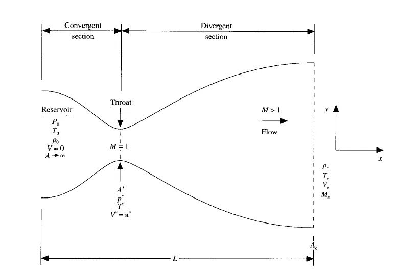
At the throat area, A=A*, p=p*, t=t* & v*=a* Mach number M=1. the sonic flow at the throat means that the local velocity at this location is equal to the local speed of sound and at the divergent section the flow expands isentropically to supersonic speed at the nozzle exit, where the pressure, temperature, velocity, and Mach number are Pr, Te, Ve and Me.

The flow is locally subsonic in the convergent section of the nozzle, sonic at the throat, and supersonic at the divergent along the x-axis. we make the assumption that the flow properties across any given cross-section and such flow is defined as quasi-one-dimensional flow.

Initial Condition and Nozzle Properties:

• Non-conservative form:

• Area = `1+2.2(x-1.5)^2`

• Density = 1-0.3146.x

• Temperature =1-0.2314*x

• Velocity = (0.1+1.09*x)*(T1/2)

• pressure = `p^' T^'`

• Mach number =`v^'/sqrtT^'`

Boundary Conditions:

Inlet boundary condition ar point 1, we choose a velocity v1 and calculate the velocity at point 1 by using linear extrapolation from points 2 and 3.

v(1)=2v(2)-v(3)

Supersonic outflow boundary condition:

v(n)=2v(n-1)-v(n-2)

p(n)=2p(n-1)-p(n-2)

t(n)=2t(n-1)-t(n-2)

Calculation of the time steps:

Timestep,`trianglet=C((trianglex)/(a+v))`

`trianglet = Timestep`

C=CFL number and we set it at 0.5

For Non-Conservative governing Equation:

Continuity Equation: `((delrho^')/(delt))=-rho^'((delv^')/(delx))-rhoV((lnA^')/(delx))-V((delrho^')/(delx))`

Momentum Equation: `((delv^')/(delt^'))=-v^'((delv^')/(delx))-1/gamma((delT^')/(delx^')+T^'/rho^'+((delT)/(delx^')))`

Energy Equation: `(delT^')/(delt^')=-V((delT^')/(delx^'))-(gamma-1)T^'[((delv^')/(delx^')+V((lnA)/(delx^'))]`

For compiling the non-conservative form we start with:

• Number of grids: The grid points distribution along with the nozzle, it is to define that the number of points along the x-axis. Form this point the characteristics of the flow are towards the right side the nozzle subsonic to supersonic
• Mesh: It is a difference between any two grid points and it will be denoted as dx. If the mesh size is smaller, the error is also small.
• Discretization: In this discretization part, we going to apply MacCormack's techniques to find the solution for conservative and non-conservative forms of 1D supersonic nozzle flow. We use the differential equation to solve explicitly for the flow field variable at time t+dt.

The MacCormack method has the following steps:

• Predictor Step
• Corrector Step
• Averaging the predictor and corrector results
• Final solution update

After the predictor step solution has to be updated.

Averaging the predictor and corrector step

`(delrho)/(delt)=0.5[((delrho)/(delt))^i+((delrho)/(delt))^(t+trianglet) i]`

Final Update:

`(rho^(t+trianglet) i) = rho^t+((delrho)/(delt))trianglet`

MATLAB FUNCTION CODE:

function [v_init,rho_init,t_init,m,M_init,p_init,rho_t,t_t,m_t,mach_t,pr_t,rho_res,t_res,v_res]=conservative_formF(x,n,nt,dx)
tic

% initial parameters
n=31;
L=3;
x=linspace(0,L,n);
dx=x(2)-x(1);
cfl=0.5;
%Area
a=1+2.2*(x-1.5).^2;

%Initial Conditions for density and tempeartures

for p=1:n
if (x(p)>=0 && x(p)<=0.5)
rho_init(p)=1;
t_init(p)=1;
else if (x(p)>=0.5 && x(p)<=1.5)
rho_init(p)=1-0.366*(x(p)-0.5);
t_init(p)=1-0.167*(x(p)-0.5);
else if (x(p)>=1.5 && x(p)<=3.5)
rho_init(p)=0.634-0.3879*(x(p)-1.5);
t_init(p)=0.833-0.3507*(x(p)-1.5);
end
end
end
end

%Velocity
v_init=0.59./(rho_init.*a);
G=1.4;
throat=find(a==1);

%vector parameters
pr=rho_init.*t_init;
u1=rho_init.*a;
u2=rho_init.*a.*v_init;
u3=u1.*((t_init./(G-1))+((G/2).*(v_init.^2)));

%claculating time step
dt=min(cfl.*(dx./((t_init.^0.5)+v_init)));

%number of cycles
nt=1400;

for k=1:nt
u1_old=u1;
u2_old=u2;
u3_old=u3;

%Flux values
f1=u2;
term=(((G-1)/G)*(u3-((G/2)*((u2.^2)./u1))));
f2=((u2.^2)./u1)+term;
f3=((G*u2.*u3)./u1)-(G*(G-1)*(u2.^3))./(2*u1.^2);

%predictor step
for i=2:n-1
df1dx(i)=(f1(i+1)-f1(i))/dx;
df2dx(i)=(f2(i+1)-f2(i))/dx;
df3dx(i)=(f3(i+1)-f3(i))/dx;

dadx(i)=(a(i+1)-a(i))/dx;
j2(i)=(1/G)*(rho_init(i)*t_init(i))*dadx(i);

%continuity equation
du1dt_p(i)=-df1dx(i);

%momentum equation
du2dt_p(i)=-df2dx(i)+j2(i);

%energy equation
du3dt_p(i)=-df3dx(i);

%solution update
u1(i)=u1(i)+du1dt_p(i)*dt;
u2(i)=u2(i)+du2dt_p(i)*dt;
u3(i)=u3(i)+du3dt_p(i)*dt;
end
rho_init=u1./a;
v_init=u2./u1;
% t_c=(G-1)*((u3./u1)-((G*u2.^2)./(2*u1)));
t_init=(G-1)*((u3./u1)-((G./2)*(v_init).^2));

%flux values for corrector step
f1=u2;
term1=(((G-1)/G)*(u3-((G./2)*((u2.^2)./u1))));
f2=((u2.^2)./u1)+term1;
f3=((G*u2.*u3)./u1)-(G*(G-1)*(u2.^3))./(2*u1.^2);

%corrector step
for l=2:n-1
df1dx(l)=(f1(l)-f1(l-1))/dx;
df2dx(l)=(f2(l)-f2(l-1))/dx;
df3dx(l)=(f3(l)-f3(l-1))/dx;

dadx1(l)=(a(l)-a(l-1))/dx;
j3(l)=(1/G)*(rho_init(l)*t_init(l))*dadx1(l);

%continuity equation
du1dt_c(l)=-df1dx(l);
%momentum equation
du2dt_c(l)=-df2dx(l)+j3(l);
%energy equation
du3dt_c(l)=-df3dx(l);

end

%Averageing values
du1dt=0.5*(du1dt_p+du1dt_c);
du2dt=0.5*(du2dt_p+du2dt_c);
du3dt=0.5*(du3dt_p+du3dt_c);

%solution update
for j=2:n-1
u1(j)=u1_old(j)+du1dt(j)*dt;
u2(j)=u2_old(j)+du2dt(j)*dt;
u3(j)=u3_old(j)+du3dt(j)*dt;

end

%Applying the boundary conditions
%inlet
u1(1)=rho_init(1)*a(1);
% velocity
u2(1)=2*u2(2)-u2(3);
%updating u3
u3(1)=u1(1)*((t_init(1)/(G-1))+((G/2)*v_init(1)^2));

%outlet
u1(n)=2*u1(n-1)-u1(n-2);
u2(n)=2*u2(n-1)-u2(n-2);
u3(n)=2*u3(n-1)-u3(n-2);

%primitive terms
rho_init=u1./a;
v_init=u2./u1;
t_init=(G-1)*((u3./u1)-((G*v_init.^2)/2));

%claculating solution
m=rho_init.*v_init.*a;
% m=v./(t.^0.5);
M_init=v_init./((t_init).^0.5);
p_init=rho_init.*t_init;

%throat values
rho_t(k)=rho_init(throat);
t_t(k)=t_init(throat);
pr_t(k)=p_init(throat);
mach_t(k)=M_init(throat);
v_t(k)=v_init(throat);
m_t(k)=m(throat);

%residual convergence
rho_res(k)=du1dt(throat);
t_res(k)=du2dt(throat);
v_res(k)=du3dt(throat);

% Exact Solution
rho_exact_n=0.634*ones(1,1400);
t_exact_n=0.833*ones(1,1400);
p_exact_n=0.528*ones(1,1400);
M_exact_n=1*ones(1,1400);

%plottings
figure(1);
if k==50
plot(x,m,'b','linewidth',2)
hold on
else if k==100
plot(x,m,'r','linewidth',2)
hold on
else if k==150
plot(x,m,'c','linewidth',2)
hold on
else if k==200
plot(x,m,'g','linewidth',2)
hold on
else if k==550
plot(x,m,'y','linewidth',2)
hold on
else if k==700
plot(x,m,'k','linewidth',2)
hold on
else if k==1400
plot(x,m,'m','linewidth',2)
hold on
grid on
xlabel('Non-dimensional Nozzle flow','fontsize',11)
ylabel('Non-dimesional Mass flow rate','fontsize',11)
legend({'50dt','100dt','150dt','200dt','550dt','700dt','1400dt'});
end
end
end
end
end
end

end

end
time=toc;
figure(3)
subplot(4,1,1)
plot(rho_t,'b')
hold on
plot(rho_exact_n,'r')
xlabel('Time Step')
ylabel('rho/{rho_0}')
legend('Time wise variation','Exact solution')
title('Time wise variation of density, Temperature, Pressure,')
grid on
subplot(4,1,2)
plot(t_t)
grid on
hold on
plot(t_exact_n,'r')
xlabel('Time Step')
ylabel('T/{T_0}')
legend('Time wise variation','Exact solution')
title('Time wise variation of density, Temperature, Pressure,')
grid on
hold on
subplot(4,1,3)
plot(pr_t)
grid on
hold on
plot(p_exact_n,'r')
xlabel('Time Step')
ylabel('P/{P_0}')
legend('Time wise variation','Exact solution')
title('Time wise variation of density, Temperature, Pressure,')
grid on
hold on
subplot(4,1,4)
plot(mach_t)
grid on
hold on
plot(M_exact_n,'r')
xlabel('Time Step')
ylabel('M/{M_0}')
legend('Time wise variation','Exact solution')
title('Time wise variation of density, Temperature, Pressure,')
grid on
hold on

figure(4)
plot(rho_res)
hold on
plot(t_res)
hold on
plot(v_res)
hold on
grid on
hold off
xlabel('Time Step')
ylabel('Density, Temperature, Velocity')
title('Residual convergence flow')
legend('Density','Temperature','Velocity')
end

*************************************************************************************************************************

Here we compile for Conservative Method:

The Initial conditions are

for `0<=x^'<=0.5 {rho^' = 1.0, T^'=1.0`

for `0.5<=x^'<=1.5{rho^' = 1.0 - 0.366(x^' - 0.5), T^' = 1.0 - 0.167(x^' - 0.5)`

for `1.5<=x^'<=3.5{rho^' = 0.634 - 0.3879(x^' - 1.5),T^' = 0.833-0.3507(x^' - 1.5)`

The subsonic conditions

u1 = `rho^'A^'`

u2=`rho^'A^'V^'`

u3=`rho^'(T^'/(gamma-1)- (gamma/2)v^('2))`

Flux terms
F1=`rho^'A^'v^'`

F2=`rho^'A^'v^('2)+((1)/(gamma )p^'A^' )`

F3=`p^'((e^')/(gamma-1)-gamma/2v^('2))v^'A^'+P^'A^'v^'`

In the Conservative form, we have an additional term called source term

J2=`(1/gamma)p^'((delA^')/(delx^'))`

The formulas for Continuity, Momentum, and Energy equations are as follows:

`((delu1)/(delt^'))= -((delF1)/(delx^'))`

Momentum Equation

`((delu2)/(delt^'))=-((delF2)/(delx^'))+J2`

Energy Equation

`((delu3)/(delt^'))=-((delF3)/(delx^'))`

The primitive variables:

`rho^'=u1/A`

`V^'=(u2/u1)`

`T^'=e^'=(gamma-1)((u3)/(u1)-gamma/2 V^('2))`

`p^' =p^'T^'`

M=`sqrtu/T`

MATLAB FUNCTION CODE:

function [v_init,rho_init,t_init,m,M_init,p_init,rho_t,t_t,m_t,mach_t,pr_t,rho_resc,t_resc,v_resc]=conservative_formF(x,n,nt,dx)
tic

% initial parameters
n=31;
L=3;
x=linspace(0,L,n);
dx=x(2)-x(1);
cfl=0.5;
%Area
a=1+2.2*(x-1.5).^2;

%Initial Conditions for density and tempeartures

for p=1:n
if (x(p)>=0 && x(p)<=0.5)
rho_init(p)=1;
t_init(p)=1;
else if (x(p)>=0.5 && x(p)<=1.5)
rho_init(p)=1-0.366*(x(p)-0.5);
t_init(p)=1-0.167*(x(p)-0.5);
else if (x(p)>=1.5 && x(p)<=3.5)
rho_init(p)=0.634-0.3879*(x(p)-1.5);
t_init(p)=0.833-0.3507*(x(p)-1.5);
end
end
end
end

%Velocity
v_init=0.59./(rho_init.*a);
G=1.4;
throat=find(a==1);

%vector parameters
pr=rho_init.*t_init;
u1=rho_init.*a;
u2=rho_init.*a.*v_init;
u3=u1.*((t_init./(G-1))+((G/2).*(v_init.^2)));

%claculating time step
dt=min(cfl.*(dx./((t_init.^0.5)+v_init)));

%number of cycles
nt=1400;

for k=1:nt
u1_old=u1;
u2_old=u2;
u3_old=u3;

%Flux values
f1=u2;
term=(((G-1)/G)*(u3-((G/2)*((u2.^2)./u1))));
f2=((u2.^2)./u1)+term;
f3=((G*u2.*u3)./u1)-(G*(G-1)*(u2.^3))./(2*u1.^2);

%predictor step
for i=2:n-1
df1dx(i)=(f1(i+1)-f1(i))/dx;
df2dx(i)=(f2(i+1)-f2(i))/dx;
df3dx(i)=(f3(i+1)-f3(i))/dx;

dadx(i)=(a(i+1)-a(i))/dx;
j2(i)=(1/G)*(rho_init(i)*t_init(i))*dadx(i);

%continuity equation
du1dt_p(i)=-df1dx(i);

%momentum equation
du2dt_p(i)=-df2dx(i)+j2(i);

%energy equation
du3dt_p(i)=-df3dx(i);

%solution update
u1(i)=u1(i)+du1dt_p(i)*dt;
u2(i)=u2(i)+du2dt_p(i)*dt;
u3(i)=u3(i)+du3dt_p(i)*dt;
end
rho_init=u1./a;
v_init=u2./u1;
% t_c=(G-1)*((u3./u1)-((G*u2.^2)./(2*u1)));
t_init=(G-1)*((u3./u1)-((G./2)*(v_init).^2));

%flux values for corrector step
f1=u2;
term1=(((G-1)/G)*(u3-((G./2)*((u2.^2)./u1))));
f2=((u2.^2)./u1)+term1;
f3=((G*u2.*u3)./u1)-(G*(G-1)*(u2.^3))./(2*u1.^2);

%corrector step
for l=2:n-1
df1dx(l)=(f1(l)-f1(l-1))/dx;
df2dx(l)=(f2(l)-f2(l-1))/dx;
df3dx(l)=(f3(l)-f3(l-1))/dx;

dadx1(l)=(a(l)-a(l-1))/dx;
j3(l)=(1/G)*(rho_init(l)*t_init(l))*dadx1(l);

%continuity equation
du1dt_c(l)=-df1dx(l);
%momentum equation
du2dt_c(l)=-df2dx(l)+j3(l);
%energy equation
du3dt_c(l)=-df3dx(l);

end

%Averageing values
du1dt=0.5*(du1dt_p+du1dt_c);
du2dt=0.5*(du2dt_p+du2dt_c);
du3dt=0.5*(du3dt_p+du3dt_c);

%solution update
for j=2:n-1
u1(j)=u1_old(j)+du1dt(j)*dt;
u2(j)=u2_old(j)+du2dt(j)*dt;
u3(j)=u3_old(j)+du3dt(j)*dt;

end

%Applying the boundary conditions
%inlet
u1(1)=rho_init(1)*a(1);
% velocity
u2(1)=2*u2(2)-u2(3);
%updating u3
u3(1)=u1(1)*((t_init(1)/(G-1))+((G/2)*v_init(1)^2));

%outlet
u1(n)=2*u1(n-1)-u1(n-2);
u2(n)=2*u2(n-1)-u2(n-2);
u3(n)=2*u3(n-1)-u3(n-2);

%primitive terms
rho_init=u1./a;
v_init=u2./u1;
t_init=(G-1)*((u3./u1)-((G*v_init.^2)/2));

%claculating solution
m=rho_init.*v_init.*a;
% m=v./(t.^0.5);
M_init=v_init./((t_init).^0.5);
p_init=rho_init.*t_init;

%throat values
rho_t(k)=rho_init(throat);
t_t(k)=t_init(throat);
pr_t(k)=p_init(throat);
mach_t(k)=M_init(throat);
v_t(k)=v_init(throat);
m_t(k)=m(throat);

%residual convergence
rho_resc(k)=du1dt(throat);
t_resc(k)=du2dt(throat);
v_resc(k)=du3dt(throat);

% Exact Solution
rho_exact_n=0.634*ones(1,1400);
t_exact_n=0.833*ones(1,1400);
p_exact_n=0.528*ones(1,1400);
M_exact_n=1*ones(1,1400);

%plottings
figure(1);
if k==50
plot(x,m,'b','linewidth',2)
hold on
else if k==100
plot(x,m,'r','linewidth',2)
hold on
else if k==150
plot(x,m,'c','linewidth',2)
hold on
else if k==200
plot(x,m,'g','linewidth',2)
hold on
else if k==550
plot(x,m,'y','linewidth',2)
hold on
else if k==700
plot(x,m,'k','linewidth',2)
hold on
else if k==1400
plot(x,m,'m','linewidth',2)
hold on
grid on
xlabel('Non-dimensional Nozzle flow','fontsize',11)
ylabel('Non-dimesional Mass flow rate','fontsize',11)
title('Mass Flow Rate')
legend({'50dt','100dt','150dt','200dt','550dt','700dt','1400dt'});
end
end
end
end
end
end

end

end
time=toc;

end

***************************************************************************************

function[rho,t,v,a,M,p,mfr,rho_res_nc,t_res_nc,v_res_nc,rho_th,t_th,p_th,M_th]=non_conservative_formF(x,n,nt,dx)
tic
clear all
close all
clc

% Length of Nozzle
L=3;
n=31;
x=linspace(0,3,n);
dx=x(2)-x(1);
gamma=1.4; %gamma
G=1.4;
% Initial Conditions
rho=1-0.3146*x; %density
t=1-0.2314*x; %Temperature
v=(0.1+1.09*x).*t.^0.5; %velocity
a=1+2.2*(x-1.5).^2;

% Throttle Values
th=(n-1)./2;
% th=find(a==1);

% Courant Number
cfl=0.5;
for z=1:n
dt(z)=cfl*((dx)/((t(z)).^0.5+(v(z))));
end
dt=min(dt);
% dt = 0.001;
nt=1400;

% Time Loop
for k=1:nt
rho_old=rho;
t_old=t;
v_old=v;
% Forward Differencing Predictor Step
for i=2:n-1

% drho_dt_P = -rho(j)*(v(j+1)-v(j))/dx -rho(j)*v(j)*(log(a(j+1))-log(a(j)))/dx -v(j)*(rho(j+1)-rho(j))/dx;
dvdx=(v(i+1)-v(i))/dx;
drhodx=(rho(i+1)-rho(i))/dx;
dtdx = (t(i+1)-t(i))/dx;
dlogadx = (log(a(i+1))-log(a(i)))/dx;

% Continuity equation
drhodt_p(i) = -rho(i)*dvdx -(rho(i)*v(i)*dlogadx) -v(i)*drhodx;

% Momentum equation
dvdt_p(i) = -v(i)*dvdx -(1/gamma)* ((dtdx) + ((t(i)/rho(i))*drhodx));

% Enerfy equation
dtdt_p(i) = -v(i)*dtdx-(gamma-1)*t(i)*((dvdx) + (v(i)*dlogadx));

% Solution update
rho(i) =rho_old(i)+drhodt_p(i)*dt;
v(i) =v_old(i)+dvdt_p(i)*dt;
t(i) =t_old(i)+dtdt_p(i)*dt;
end
for j=2:n-1
dvdx=(v(j)-v(j-1))/dx;
drhodx=(rho(j)-rho(j-1))/dx;
dtdx = (t(j)-t(j-1))/dx;
dlogadx = (log(a(j))-log(a(j-1)))/dx;

% Continuity equation
drhodt_c(j) = -rho(j)*dvdx -(rho(j)*v(j)*dlogadx) -v(j)*drhodx;

% Momentum equation
dvdt_c(j) = -v(j)*dvdx -(1/gamma)* ((dtdx) + ((t(j)/rho(j))*drhodx));

% Enerfy equation
dtdt_c(j) = -v(j)*dtdx-(gamma-1)*t(j)*((dvdx) + (v(j)*dlogadx));

end
% Compute the average time derivative
drhodt = 0.5*(drhodt_p + drhodt_c);
dvdt = 0.5*(dvdt_p + dvdt_c);
dtdt = 0.5*(dtdt_p +dtdt_c);

% Averaging
drhodt_avg=(0.5*dt*(drhodt_p+drhodt_c));
dtdt_avg=(0.5*dt*(dtdt_p+dtdt_c));
dvdt_avg=(0.5*dt*(dvdt_p+dvdt_c));
for m=2:n-1

rho(m)=rho_old(m)+drhodt_avg(m);
t(m)=t_old(m)+dtdt_avg(m);
v(m)=v_old(m)+dvdt_avg(m);
end
% Boundary Conditions
% Intelt
v(1)=(2*v(2))-v(3);
% Outlet
v(n)=(2*v(n-1))-v(n-2);
t(n)=(2*t(n-1))-t(n-2);
rho(n)=(2*rho(n-1))-rho(n-2);

% Pressure Ratio
p=rho.*t;

% Mach Number
M=v./(t.^0.5);

% Mass FLow Rate
mfr=rho.*v.*a;

% Throttle values
rho_th(k)=rho(th);
t_th(k)=t(th);
p_th(k)=p(th);
M_th(k)=M(th);

% Throttle residual values
rho_res_nc(k)=drhodt_avg(th);
t_res_nc(k)=dtdt_avg(th);
v_res_nc(k)=dvdt_avg(th);

figure(2)
hold on
if k==1
plot(x,mfr,'linewidth',2)
grid on
else if k==50
plot(x,mfr,'linewidth',2)
else if k==100
plot(x,mfr,'linewidth',2)
else if k==200
plot(x,mfr,'linewidth',2)
else if k==700
plot(x,mfr,'linewidth',2)
else if k==1400
plot(x,mfr,'linewidth',2)
xlabel('Non-dimensional nozzle dimension','fontsize',11);
ylabel('Non-dimensional mass flow rate','fontsize',11);
legend('0dt','50dt','100dt','200dt','700dt','1400dt')
title('Mass Flow Rate at Different Time Step','Fontweight','bold','fontsize',11)
hold on
grid on
hold off
end
end
end
end
end
end

end

time=toc;
end

MAIN CODE FOR GETTING THE PLOTTINGS AND VALUES:

clear all
close all
clc
% inputs
n=31;
x=linspace(0,3,n);
dx=x(2)-x(1);

G=1.4;
nt=1400;

tic;
[v_init,rho_init,t_init,m,M_init,p_init,rho_t,t_t,m_t,mach_t,p_t,rho_resc,t_resc,v_resc]=conservative_formF(x,n,nt,dx);
conservative_time=toc;

hold on

tic;
[rho,t,v,a,M,p,mfr,rho_res_nc,t_res_nc,v_res_nc,rho_th,t_th,p_th,M_th]=non_conservative_formF(x,n,nt,dx);
non_conservative_time=toc;

% Exact Solution
rho_exact_n=0.634*ones(1,1400);
t_exact_n=0.833*ones(1,1400);
p_exact_n=0.528*ones(1,1400);
M_exact_n=1*ones(1,1400);

figure(3)
subplot(4,1,1)
plot(x,M,'r');
hold on
plot(x,M_init,'*');
hold on
grid on
xlabel('X')
ylabel('Mach Number')
legend('Non-Conservative','Conservative')
title(sprintf('Qualitativ Aspect of Quasi-1D Nozzle Flow'));
subplot(4,1,3)
plot(x,rho,'r');
hold on
plot(x,rho_init,'*');
hold on
grid on
xlabel('X')
ylabel('Density')
legend('Non-Conservative','Conservative')
subplot(4,1,2)
plot(x,p,'r');
hold on
plot(x,p_init,'*');
hold on
grid on
xlabel('X')
ylabel('Pressure')
legend('Non-Conservative','Conservative')
subplot(4,1,4)
plot(x,t,'r');
hold on
plot(x,t_init,'*');
hold on
grid on
xlabel('X')
ylabel('Temperature')
legend('Non-Conservative','Conservative')

figure(4)
subplot(4,1,1)
plot(rho_t,'b')
hold on
plot(rho_exact_n,'r')
grid on
grid on
xlabel('Time Step')
ylabel('rho/{rho_0}')
title('Time wise variation of Density, Pressure, Temperature, Mach Number C.F')
legend('Time wise variation','Exact Solution')

subplot(4,1,2)
plot(t_t)
hold on
plot(t_exact_n)
grid on
xlabel('Time Step')
ylabel('T/{T_0}')
legend('Time wise variation','Exact Solution')

subplot(4,1,3)
plot(p_t)
hold on
plot(p_exact_n)
grid on
xlabel('Time Step')
ylabel('P/{P_0}')
legend('Time wise variation','Exact Solution')

subplot(4,1,4)
plot(mach_t)
hold on
plot(M_exact_n)
hold on
xlabel('Time Step')
ylabel('M/{M_0}')
legend('Time wise variation','Exact Solution')

figure(5)
plot(rho_resc)
hold on
plot(t_resc)
hold on
plot(v_resc)
hold on
grid on
hold off
xlabel('Time Step')
ylabel('Density, Temperature, Velocity')
title('Residual convergence flow')
legend('Density','Temperature','Velocity')

figure(6)
subplot(4,1,1)
plot(rho_th)
hold on
plot(rho_exact_n)
grid on
xlabel('Time Step')
ylabel('rho/{rho_0}')
title('Time wise variation of Density, Pressure, Temperature, Mach Number N.C.F')
legend('Time wise variation','Exact Solution')

subplot(4,1,2)
plot(t_th)
hold on
plot(t_exact_n)
grid on
xlabel('Time Step')
ylabel('T/{T_0}')
legend('Time wise variation','Exact Solution')

subplot(4,1,3)
plot(p_th)
hold on
plot(p_exact_n)
grid on
xlabel('Time Step')
ylabel('P/{P_0}')
legend('Time wise variation','Exact Solution')

subplot(4,1,4)
plot(M_th)
hold on
plot(M_exact_n)
hold on
grid on
xlabel('Time Step')
ylabel('M/{M_0}')
legend('Time wise variation','Exact Solution')

figure(7)
plot(rho_res_nc)
hold on
plot(t_res_nc)
hold on
plot(v_res_nc)
hold on
grid on
hold off
xlabel('Time Step')
ylabel('Density, Temperature, Velocity')
title('Residual Plots NON-CONSERVATIVE')
legend('Density','Temperature','Velocity')

figure(8)
plot(x,mfr,'linewidth',2)
hold on
plot(x,m,'linewidth',2)
xlabel('X/L')
ylabel('Non-dimensional mass flow rate')
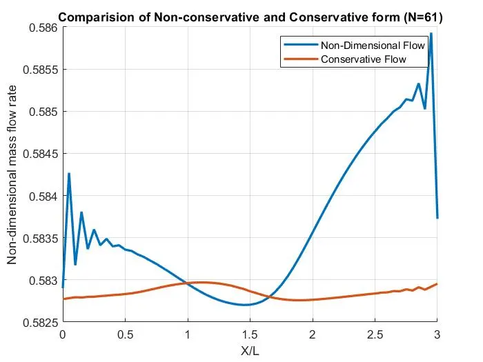
title('Comparision of Non-conservative and Conservative form (N=61)')
legend('Non-Dimensional Flow','Conservative Flow')
grid on

PICTORIAL REPRESENTATIONS

FLOW THROUGHOUT THE NOZZLE: N=31

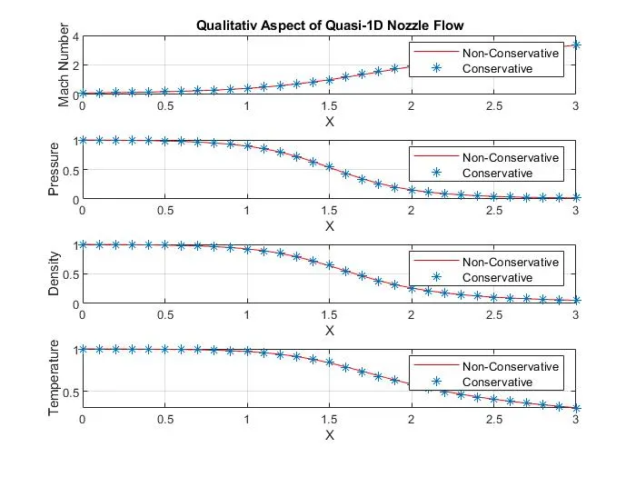
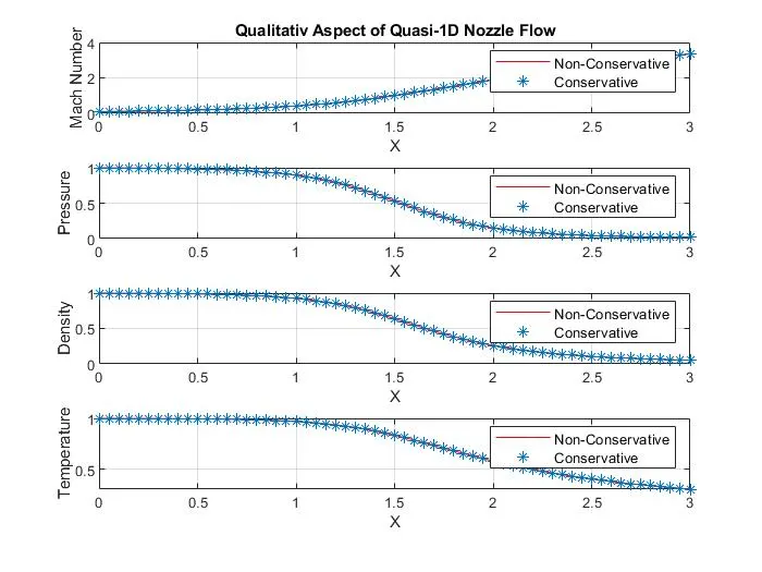
FLOW THROUGHOUT THE NOZZLE: N=61

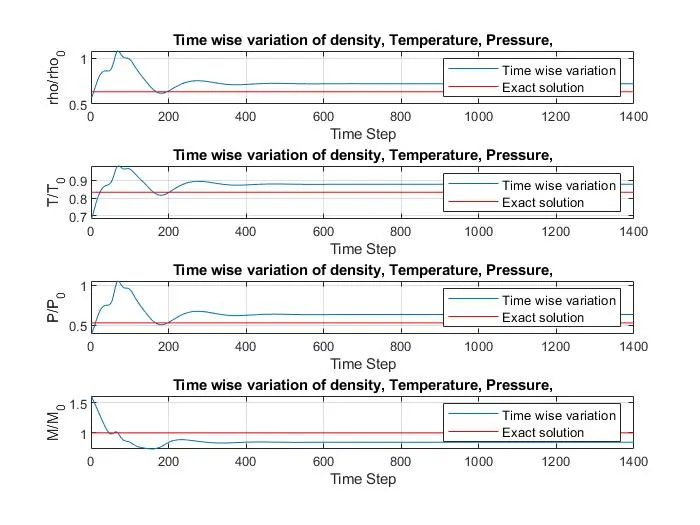
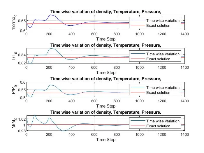
• Time Variation of Flow Parameter Along The Non-Dimensional Length of Nozzle at Throat.

1. From the above graph, it can be said that the solution of the Non-Conservative form lies closer to the exact values of density, temperature, and Mach number when compared to the conservative form solution.
2. The above values of flow parameters in a particular region are a good way of investigating the attainment of the steady-state by the system.
3. The Non-Conservative form gives the exact and accurate results of the primitive variables.

• TIME WISE VARIATION NON-CONSERVATIVE FORM N=31;

• TIME WISE VARIATION NON-CONSERVATIVE FORM N=61;

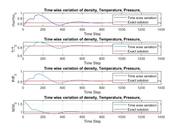
• TIME WISE VARIATION CONSERVATIVE FORM N=31;

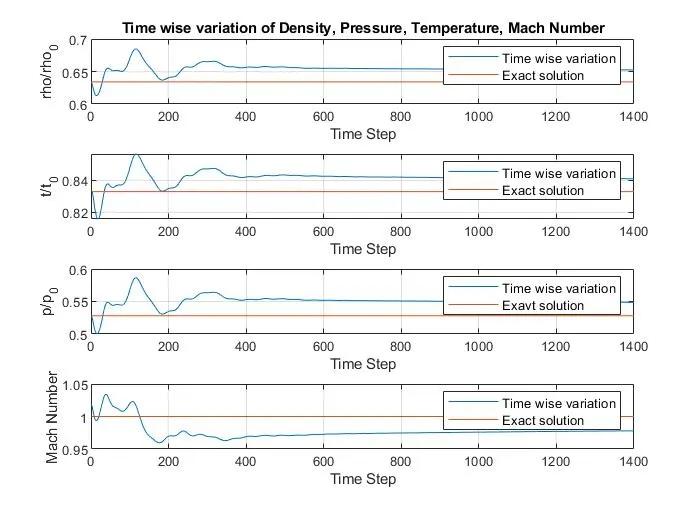
• TIME WISE VARIATION CONSERVATIVE FORM N=61;

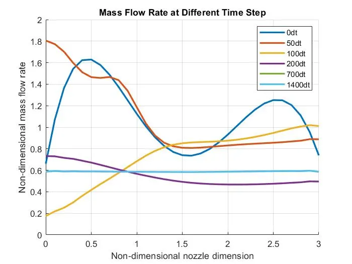
• MASS FLOW RATE NON-CONSERVATIVE FORM N=31:

• MASS FLOW RATE NON-CONSERVATIVE FORM N=61:

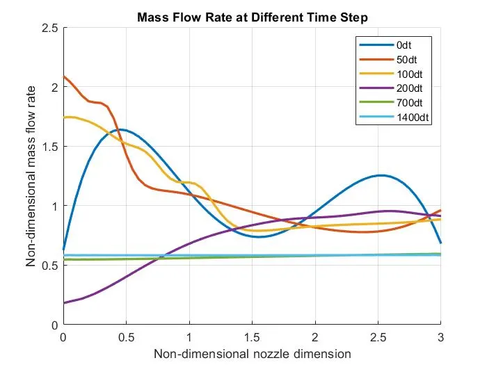
1. The mass flow rate for 1400 time steps is almost overlaying in the same region of space.
2. After 500 timesteps the plots are in the steady-state form.
3. whereas theoretically, it will take an infinite number of timesteps to obtain a steady-state form.

• MASS FLOW RATE CONSERVATIVE FORM N=31:

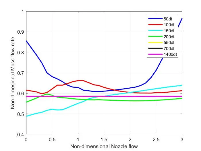
• MASS FLOW RATE CONSERVATIVE FORM N=31:

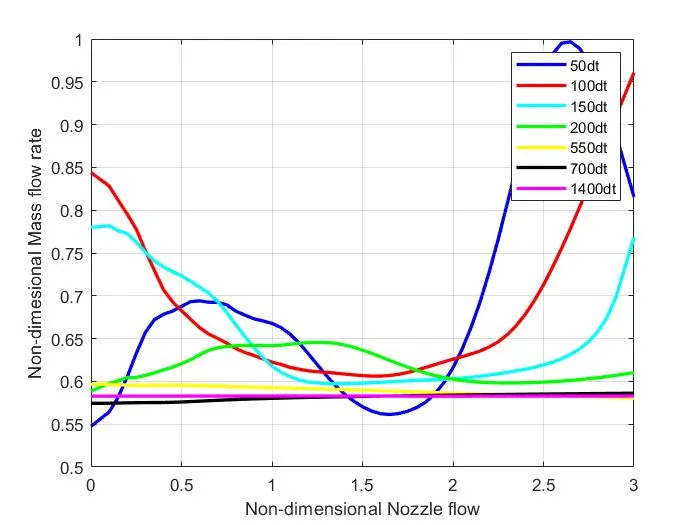
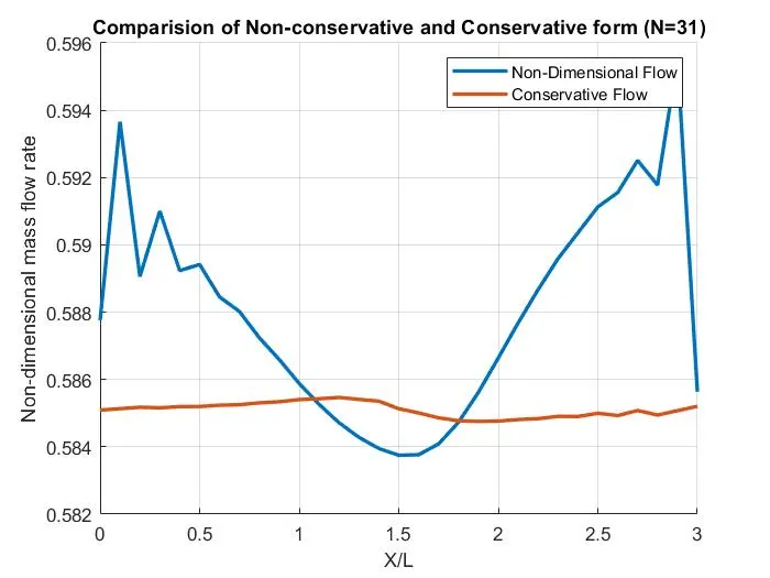
1. As we assumed the initial conditions for density, temperature and velocity with the constant mass flow for the conservative form because of its sensitive behaviour it tends to possess mild fluctuations.
2. It can be observed from the above plot that at 550,700 and 1400 timesteps are almost overlaying in the same region.

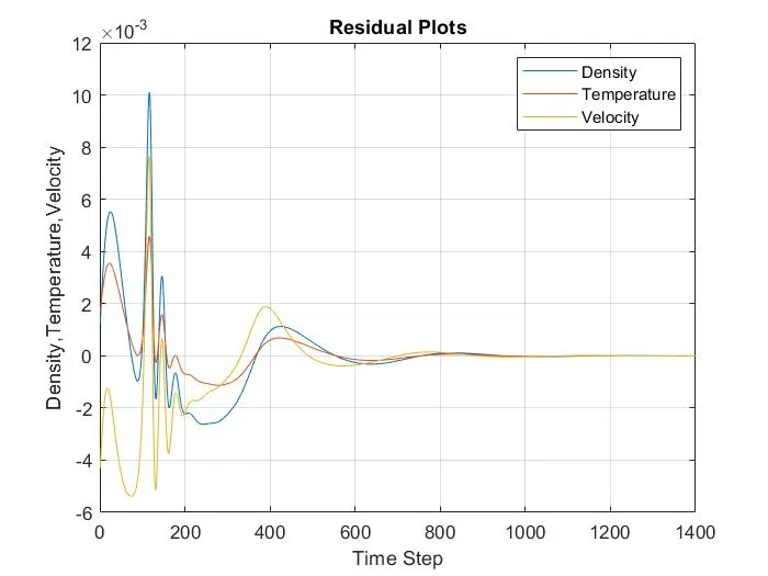
NON-CONSERVATIVE FORM RESIDUAL PLOTS(N=31)

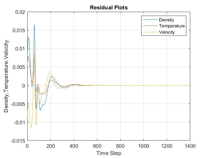
NON-CONSERVATIVE FORM RESIDUAL PLOTS(N=61)

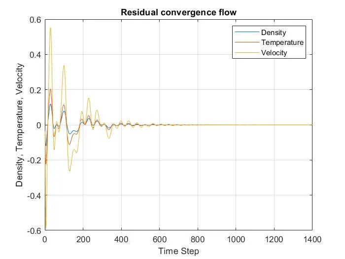
CONSERVATIVE FORM RESIDUAL PLOTS(N=31)

CONSERVATIVE FORM RESIDUAL PLOTS(N=61)

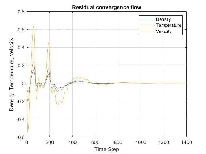
• FACTORS INFLUENCING THE RESIDUAL FLOWS:

1. Small Inflow Boundary Conditions: As we are assuming the density, temperature and pressure at the inlet are equal to the reservoir properties. This is only true if the Mach number at the inlet is equal to zero. But Mach number is a function of the area. Here it is an inbuilt error which is neglected.
2. Courant Number: According to the theory of courant number stability criteria, the CFL number should be less than or equal to 0.5. But this number is smaller necessary at which the solution. CFL criteria provide a good estimate to calculate the timestep value for nonlinear hyperbolic PDE. It may not give exact values because it derived for linear hyperbolic equations.
3. Grid Dependence: grid independence test can also be carried out by comparing the conservative and non-conservative values at the throat for n=31 and 61. It is evident that conservative and non-conservative form results tend to be accurate to the exact analytical values. Even though by doubling the number of grid points the solutions seems to be closer to the values of exact analytical values.

CODE FOR GRID DEPENDENCY TEST USING FZERO FUNCTION:

function [x,G,th,P_E,R_E,T_E,M_E]=analytical_exact_values(a,n)
n=31;
x=linspace(0,3,n);
% t=1-0.2314*x;
% v=(0.1+1.09*x).*t.^0.5;
% M=v./(t.^0.5);
G=1.4;
% Area (A/A*)
a=1+2.2*(x-1.5).^2;
th =16;
MachNo = ones(1,1400);
for i=1:31
f=@(M) ((1/M.^2)*((2/(G+1))*(1+((G-1)/2)*M.^2))^((G+1)/(G-1))-a(i)^2);
if(i<th)
x0 = [1e-4 1-1e-4];
MachNo(i) = fzero(f,x0);
disp(MachNo(i))
end

if i==th
MachNo(i) = 1;
disp(MachNo(i))
end
if i>th
x0 = [1+1e-4 10] ;
MachNo(i) = fzero(f,x0);
disp(MachNo(i))
end
end
M_E=MachNo;
P_E=(1+((G-1)/2)*M_E.^2).^(-G/(G-1));
R_E=(1+((G-1)/2)*M_E.^2).^(-1/(G-1));
T_E=(1+((G-1)/2)*M_E.^2).^-1;

end

Grid Dependency Test:

	Density	Temperature	Pressure	Mach Number
Grid's =31	0.6387	0.8365	0.5342	0.9994
Grid's =61	0.6376	0.8354	0.4823	1
Exact Analytical Values	0.6339	0.8333	0.5283	1