Week 6 - Multivariate Newton Rhapson Solver

Aim :

To solve the given set of coupled non linear equations using multivariate newton raphson method.

Given data:

Initial guess values:

y1=1

y2=0

y3=0

Methods incorporating newton raphson solver:

1. Implicit scheme

2.Jacobian method.

Newton Raphson method:

The Newton-Raphson method (also known as Newton's method) is a way to quickly find a good approximation for the root of a real-valued function f(x) = 0f(x)=0. It uses the idea that a continuous and differentiable function can be approximated by a straight line tangent to it.

Suppose you need to find the root of a continuous, differentiable function f(x)f(x), and you know the root you are looking for is near the point x = x_0x=x0​. Then Newton's method tells us that a better approximation for the root is

`x_1 = x_0 - \frac{f(x_0)}{f'(x_0)}`

This process may be repeated as many times as necessary to get the desired accuracy. In general, for any xx-value x_nxn​, the next value is given by

`x_{n+1} = x_n - \frac{f(x_n)}{f'(x_n)}`

For a multivariate equation the equation is devised as

`x_(New) = x_(guess) - alpha.J^-1.F`

where `alpha` is relaxation factor

J is the jacobian matrix.

F is the function`((f1),(f2),(f3))`the equations.

Jacobian matrix:

It is the matrix which contains all the possible derivatives of the coupled equations coressponding to the number of variables.

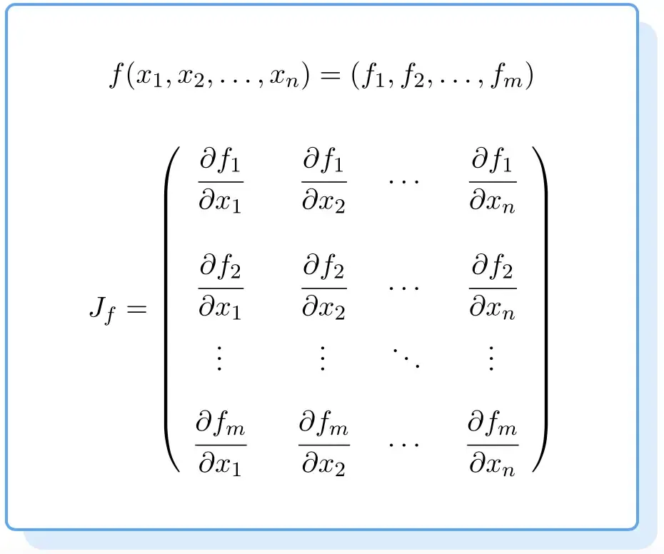
Derivation of the coupled non-linear equations are solved and uploaded in the below link

https://drive.google.com/file/d/1AWHRMkdnQ9KDG9KlNL2Linxj7FITg3NE/view?usp=sharing

And now we can use the function matrix to calculate the Jacobian matrix and solve using Newton raphson solver.

`x_(New) = x_(guess) - alpha.J^-1.F`

The code:

import numpy as np 
import matplotlib.pyplot as plt
from numpy.linalg import inv

def f1(y1,y2,y3,y_old1,h):
	return y_old1+h*(-0.04*y1 +pow(10,4)*y2*y3)-y1

def f2(y1,y2,y3,y_old2,h):
    return y_old2 +h*(0.04*y1-pow(10,4)*y2*y3-3*pow(10,7)*pow(y2,2))-y2

def f3(y1,y2,y3,y_old3,h):
    return y_old3 +h*(3*pow(10,7)*pow(y2,2))-y3

#function for Jacobian matrix
def jacobian(y_new,y_old,h):
    
    J=np.ones((3,3))

    y_old1=y_old[0]
    y_old2=y_old[1]
    y_old3=y_old[2]

    dy=1e-10
    y1=y_new[0]
    y2=y_new[1]
    y3=y_new[2]

    J[0,0]=(f1(y1+dy,y2,y3,y_old[0],h)-f1(y1,y2,y3,y_old[0],h))/dy
    J[0,1]=(f1(y1,y2+dy,y3,y_old[0],h)-f1(y1,y2,y3,y_old[0],h))/dy
    J[0,2]=(f1(y1,y2,y3+dy,y_old[0],h)-f1(y1,y2,y3,y_old[0],h))/dy
    
    J[1,0]=(f2(y1+dy,y2,y3,y_old2,h)-f2(y1,y2,y3,y_old2,h))/dy
    J[1,1]=(f2(y1,y2+dy,y3,y_old2,h)-f2(y1,y2,y3,y_old2,h))/dy
    J[1,2]=(f2(y1,y2,y3+dy,y_old2,h)-f2(y1,y2,y3,y_old2,h))/dy
    
    J[2,0]=(f3(y1+dy,y2,y3,y_old3,h)-f3(y1,y2,y3,y_old3,h))/dy
    J[2,1]=(f3(y1,y2+dy,y3,y_old3,h)-f3(y1,y2,y3,y_old3,h))/dy
    J[2,2]=(f3(y1,y2,y3+dy,y_old3,h)-f3(y1,y2,y3,y_old3,h))/dy

    return J




h=0.1
time=np.arange(0,600,h)
alpha =1


F=np.zeros((3,1))
y_old=np.zeros((3,1))
y_new =np.zeros((3,1))
y_old[0]=1
tol=1e-10
y1=[]
y2=[]
y3=[]

for i in range(0,len(time)):

    y_guess=np.copy(y_old)

    error=9e9
    while error>tol: 
        Jac=jacobian(y_new,y_old,h)
        F[0]=f1(y_guess[0],y_guess[1],y_guess[2],y_old[0],h)
        F[1]=f2(y_guess[0],y_guess[1],y_guess[2],y_old[1],h)
        F[2]=f3(y_guess[0],y_guess[1],y_guess[2],y_old[2],h)

        
        y_new=y_guess - alpha*np.matmul(inv(Jac),F)
        error=max(abs(y_new-y_guess))
        y_guess= y_new
    y_old=y_new
    y1.append(y_new[0])
    y2.append(y_new[1])
    y3.append(y_new[2])

plt.plot(time,y1,label='y1')
plt.plot(time,y2,label='y2')
plt.plot(time,y3,label='y3')
plt.legend()
plt.show()

Plots:

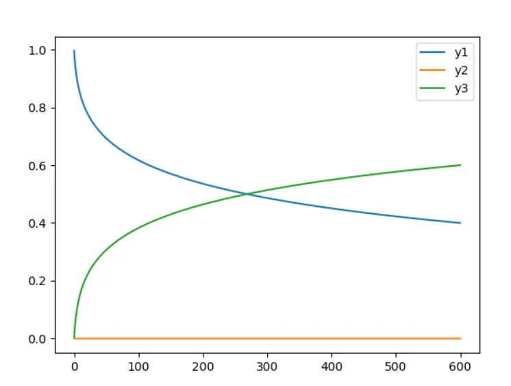
when dt =0.1

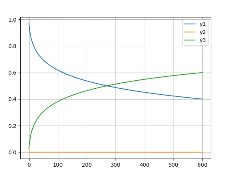
When dt=1:

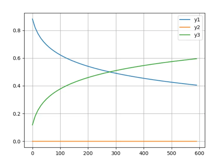
When dt =10:

About the Code:

• We write codes for the functions f1,f2,f3 and for the jacobian before the main code.
• In the main code we specify values for all the yold ,dt, error, tolerances specified.
• And we create three arrays to store the y new values and give some guess values initially as specified in the question.
• We run the for loop for 10 minutes and while loop until the error > tolerance, we calculate the ynew value using the newton raphson solver by backward differencing scheme.
• And update the value of yold and yguess at all the time steps.
• Plot the results finally.

Conclusion:

The implicit scheme is not sensitive here ,it gives almost the same results for dt values less than 1, but the solution gets disturbed when using a larger time step (dt>1). So the ideal step size would be dt=0.1.