Week 1- Mixing Tee
Aim:
To set up steady-state simulations to compare the mixing effectiveness when hot inlet temperature is 360C & the Cold inlet is at 190C.
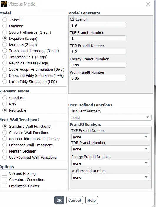
Use the k-epsilon and k-omega SST model for the first case and based on your judgment use the more suitable model for further cases.
- Case 1
- Short mixing tee with a hot inlet velocity of 3m/s.
- Momentum ratio of 2, 4.
- Case 2
- Long mixing tee with a hot inlet velocity of 3m/s.
- Momentum ratio of 2, 4.
Objectives:
- Cell count
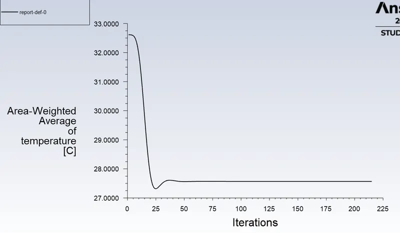
- Average outlet temperature
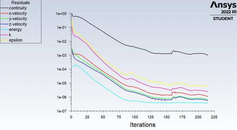
- Number of iterations for convergence
and plot the expected results of
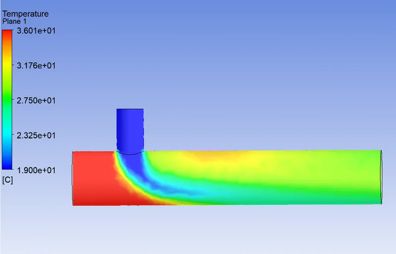
- Velocity and temperature contour plots on the cut planes along and across the pipe.
- Velocity and temperature line plots along and across the length of the pipe.
- Perform Mesh independent study for any one case.
- Discuss the effect of length and momentum ratio on results.
Procedure:
- Open the Ansys workbench and use the fluid flow (fluent) module from the analysis systems available.
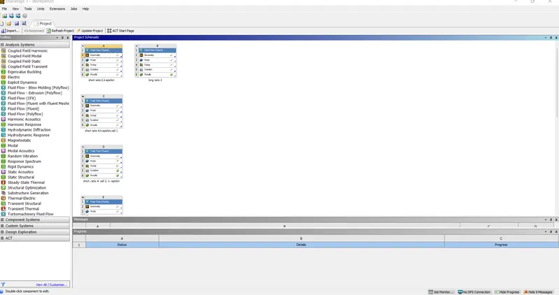
- Import the required geometry and check if the geometry is updated and use the suppress for physics option to suppress the parts of the geometry that are not actually needed for the analysis.And extract the volume in which the simulation takes place of the tee geometry using the volume extract option under prepare and exit the geometry.
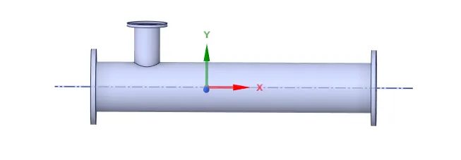
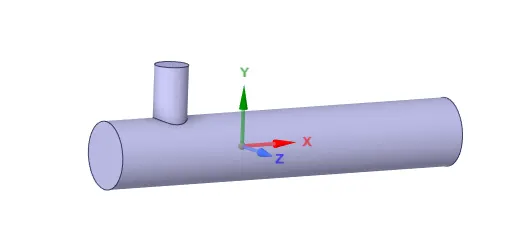
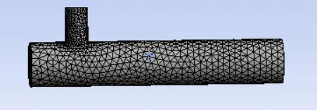
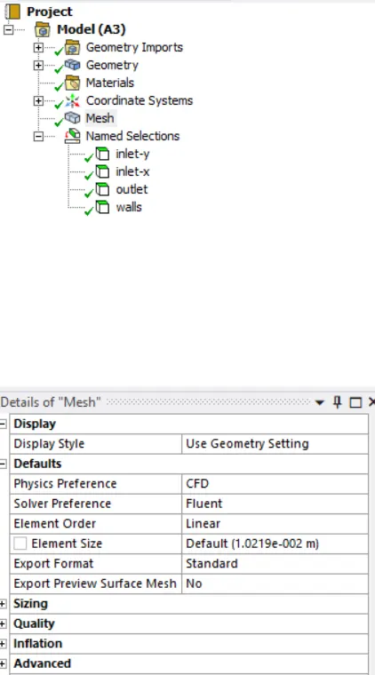
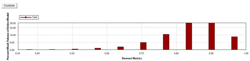
- Now select the mesh and create a named selection for the inlet ,outlet, and walls ,so that it is easier for the workbench to simulate.Then mesh the geometry by providing the required element size and use the quality of mesh detail and select the element quality to know how the mesh has been applied to the geometry and exit the mesh.
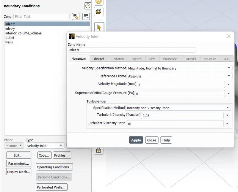
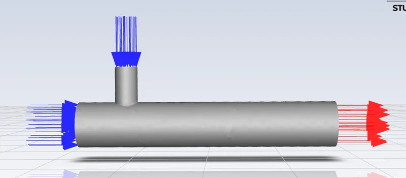
- Open the setup ,you can see the console runs to create the geometry.Now set up the physics of the simulation using the viscous model option and select the required model for the simulation. Set the boundary conditions for the inlet and outlet using the boundaries under zones. Select the energy dialog box to apply the temperature conditions in the simulation.
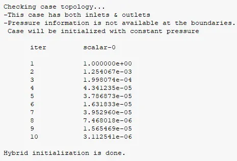
- Now under the solution select the required result you want to see by using the defenition function and select the hybrid method for the simulation and initialize t=0 nad set the required number of iterations and select calculate to start the simulation.
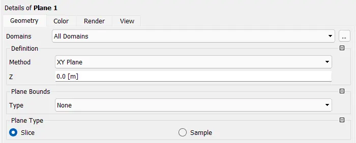
- Now then exit the setup and open the result for the post processing of the simulation results.Select only the walls and suppress all other parameters and cretae a plane in the mid of the Tee geometry and adjust the transparency of the geometry and change colour of the geometry until you feel the result is properly visible.
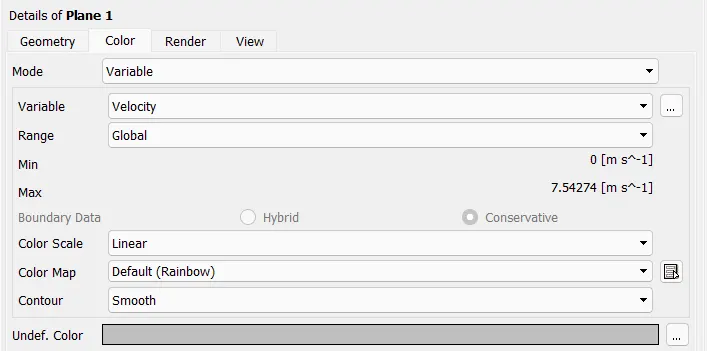
- Now then change the different variable parameters to find the results.
Results for K - epsilon method:
Short pipe
momentum ratio -2
cell count - 12613
The mesh:
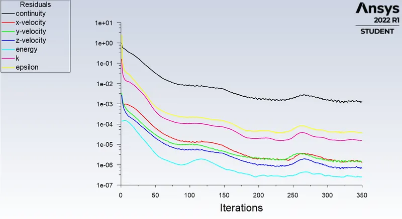
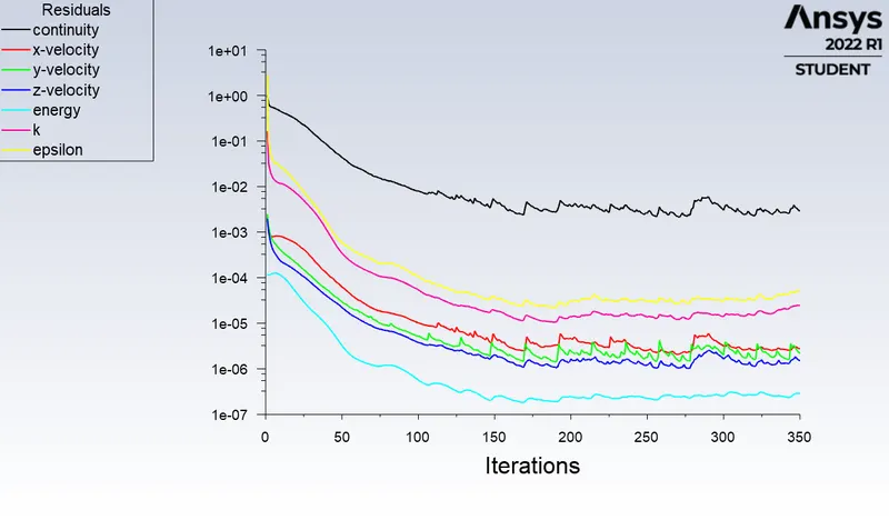
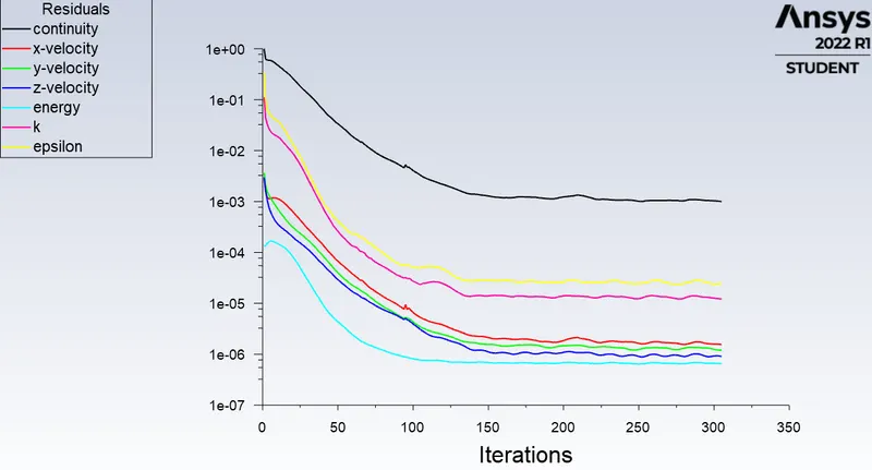
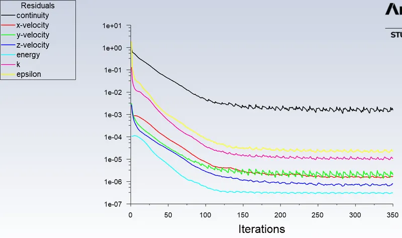
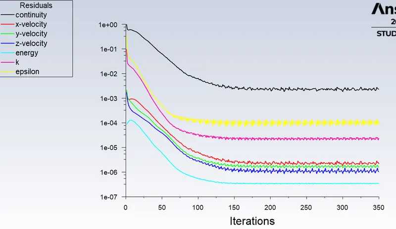
Residulas vs Iterations:
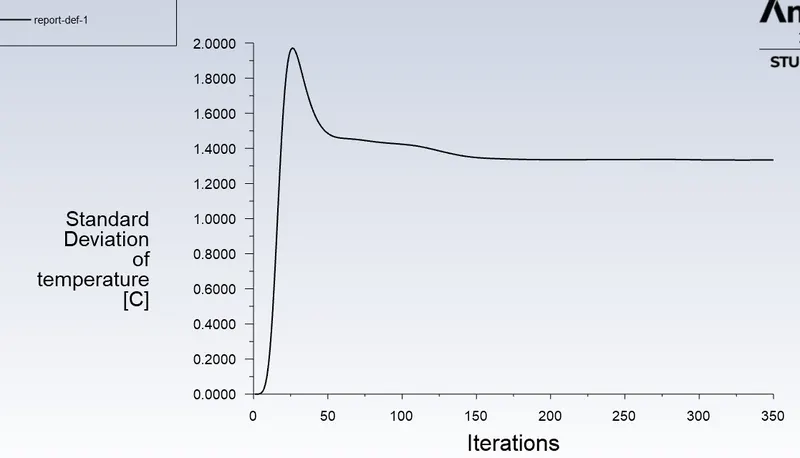
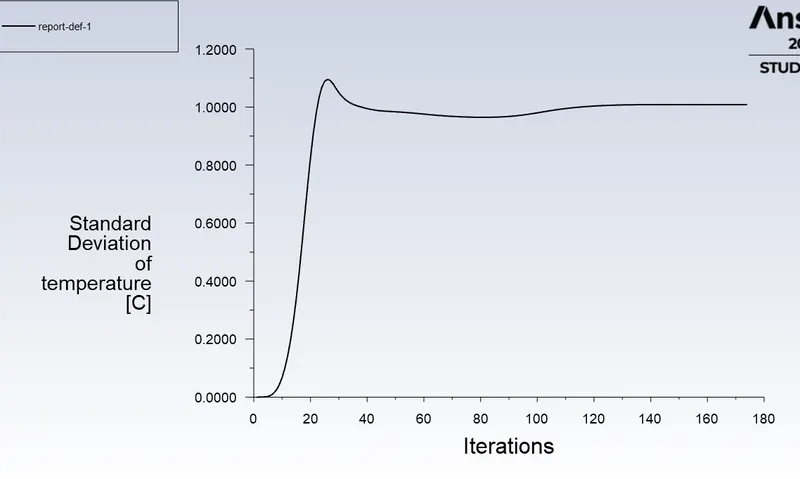
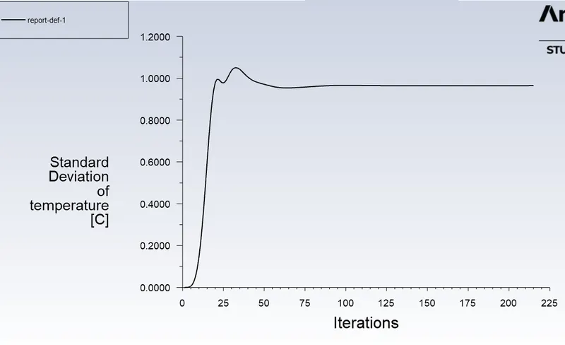
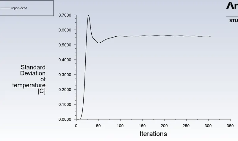
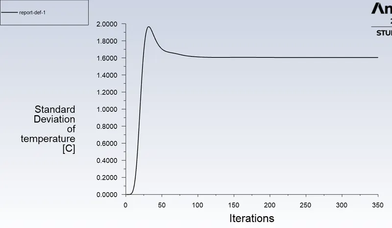
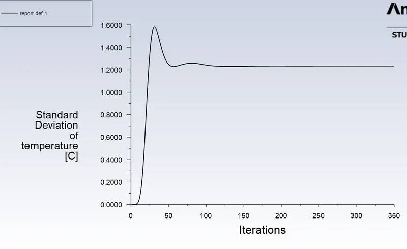
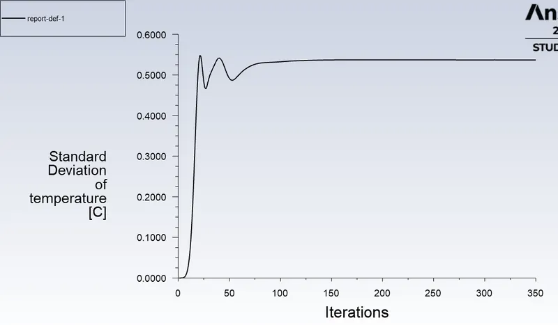
Standard deviation of temperature vs Iterations:
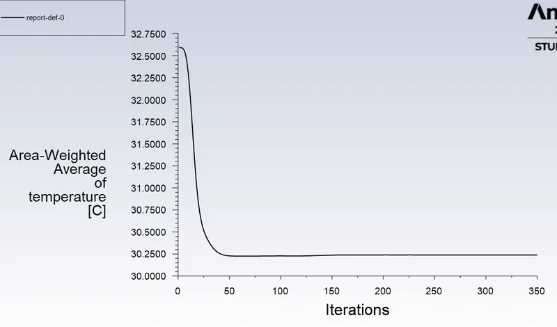
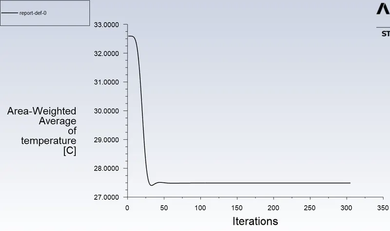
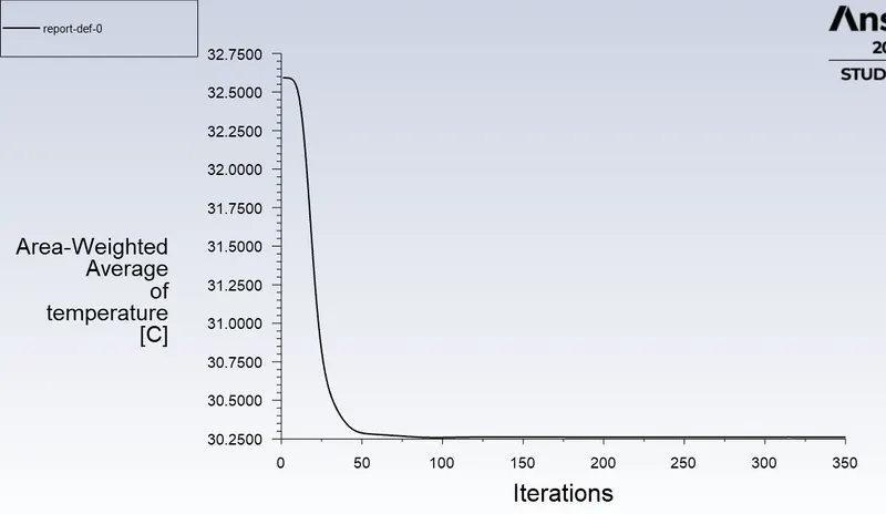
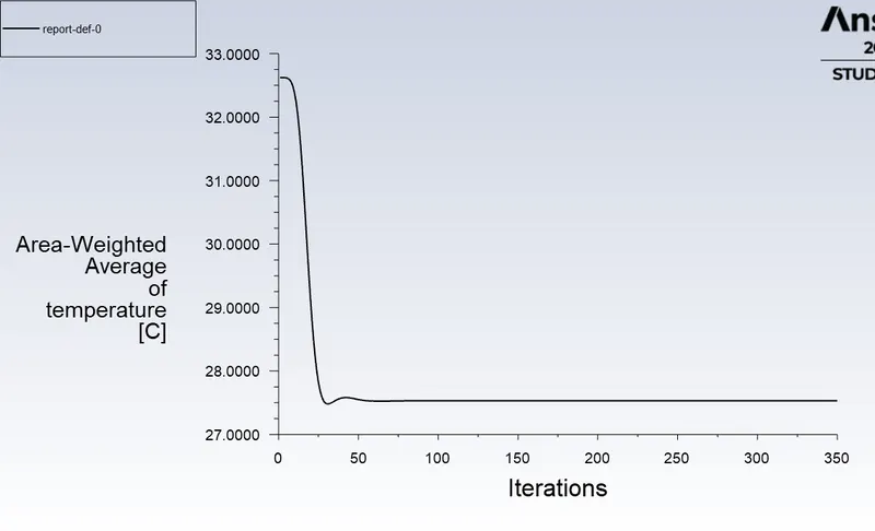
Area weighted average of temperature vs Iterations:
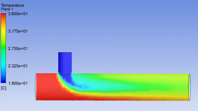
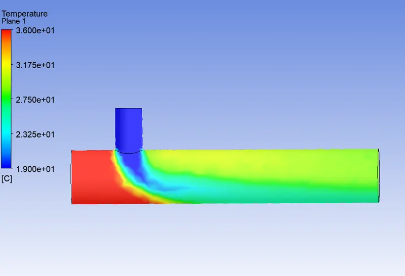
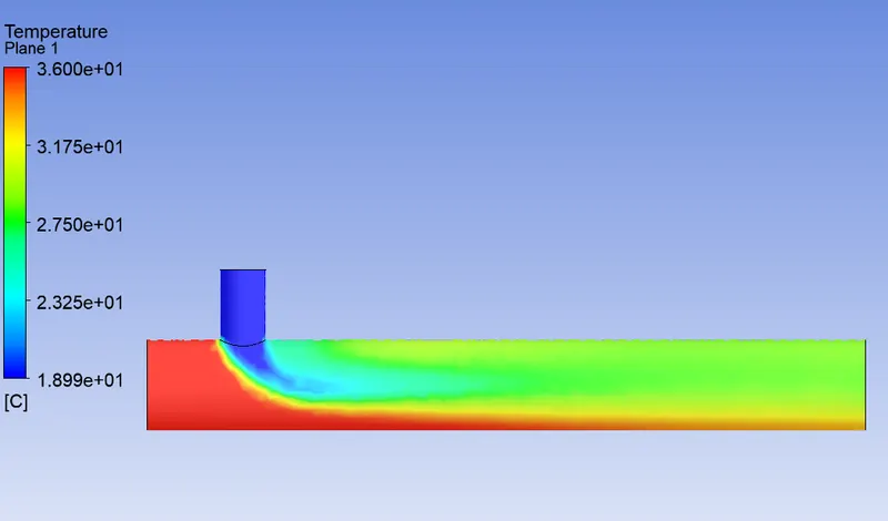
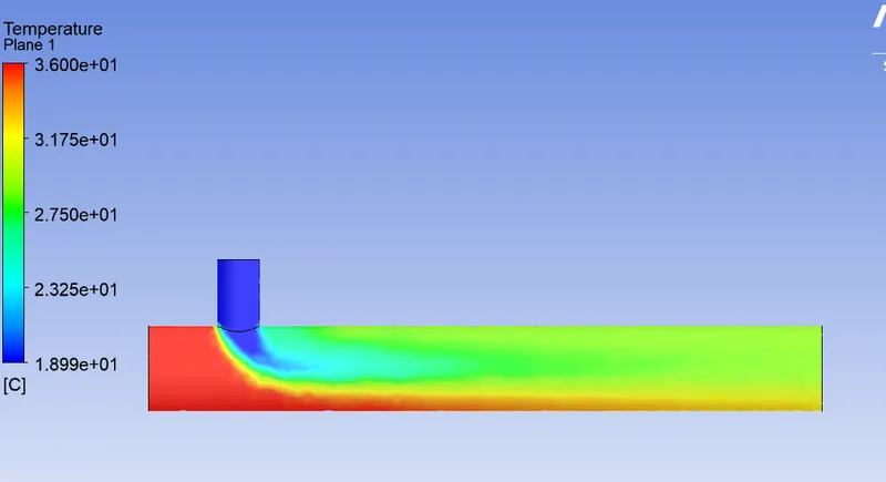
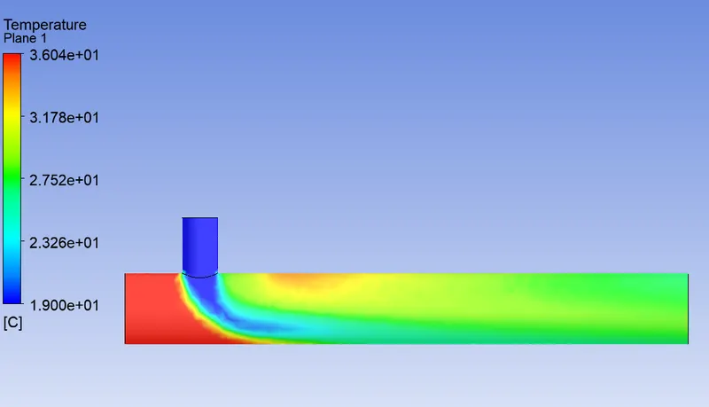
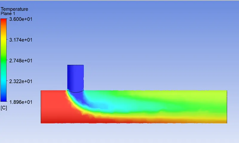
Temperature contour :
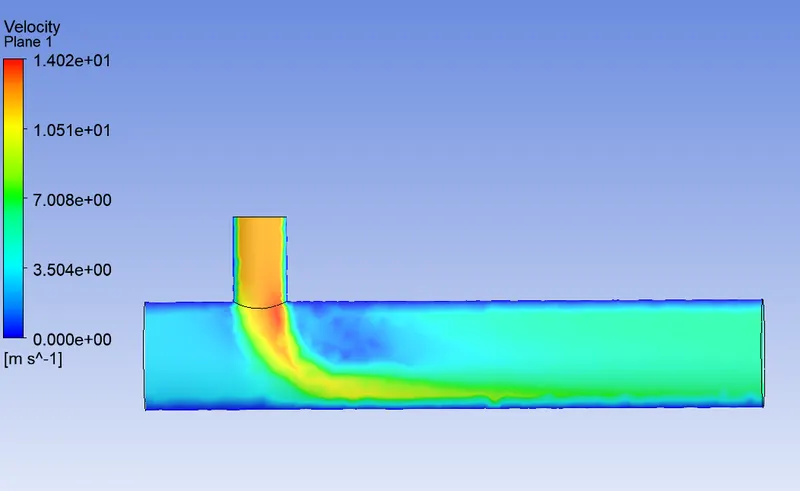
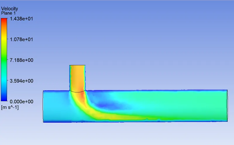
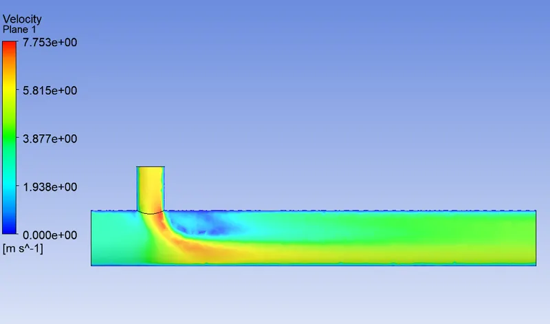
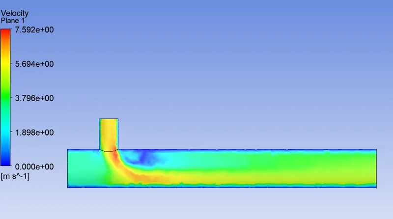
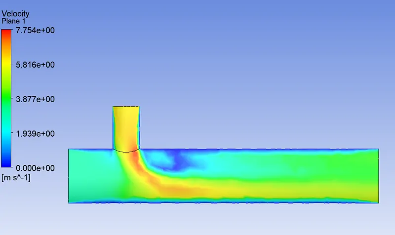
Velocity contour:
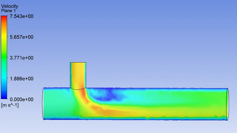
Results for K- omega method:
Short pipe
momentum ratio -2
cell count - 12613
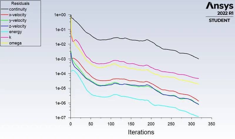
Residulas vs Iterations:
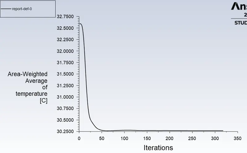
Area weighted average of temperature vs Iterations:
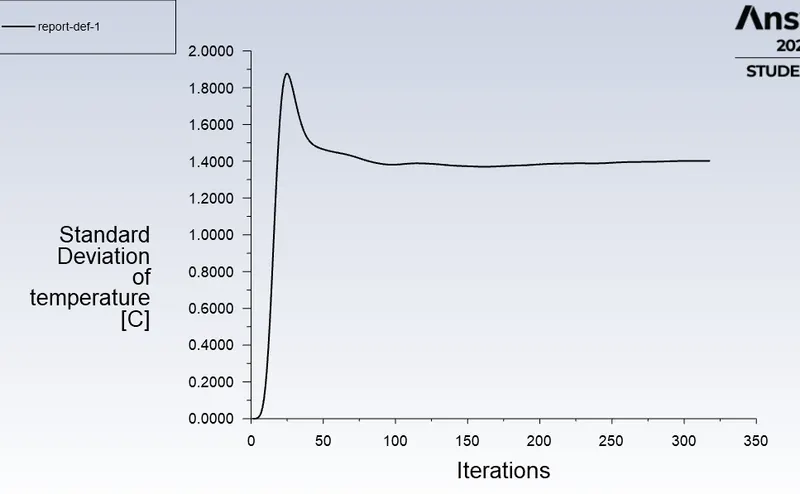
Standard deviation of temperature vs Iterations:
Temperature contour :
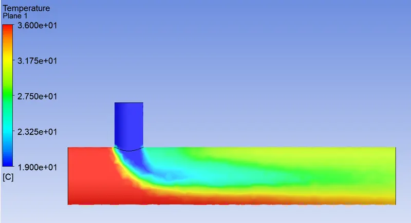
Velocity contour:
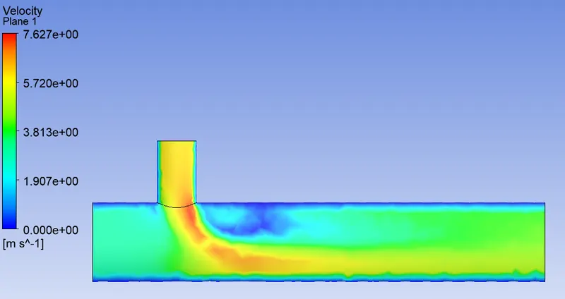
The above results represent the simulation of the geometry with k-omega sst model.
K-Epsilon:
K-epsilon (k-ε) turbulence model is the most common model used in computational fluid dynamics(CFD) to simulate mean flow characteristics for turbulent flow conditions. It is a two-equation model that gives a general description of turbulence by means of two transport equations.
K- omega:
In computational fluid dynamics, the k–omega (k–ω) turbulence model is a common two-equation turbulence model, that is used as an approximation for the Reynolds-averaged Navier–Stokes equations (RANS equations). The model attempts to predict turbulence by two partial differential equations for two variables, k and ω, with the first variable being the turbulence kinetic energy (k) while the second (ω) is the specific rate of dissipation.
Difference:
K epsilon is best suited for flow away from the wall, say free surface flow region, whereas k-omega model is best suited for near the wall flow region, where adverse pressure gradient is developed.
Short pipe
momentum ratio -4
cell count - 12613
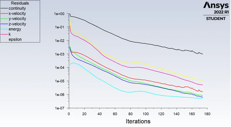
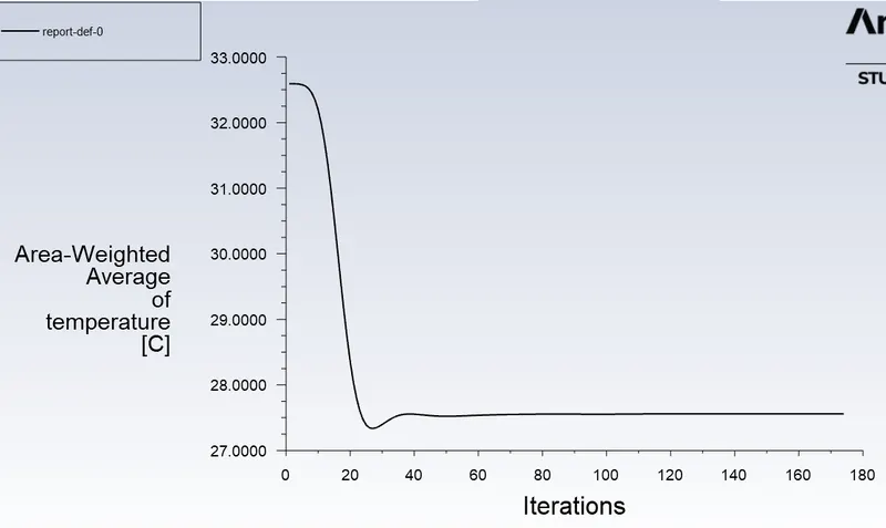
Short pipe
momentum ratio -2
cell count - 22296
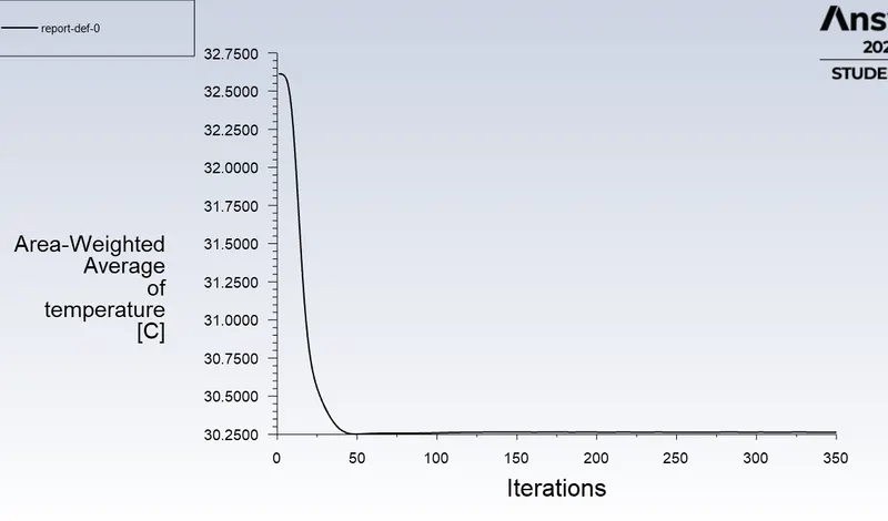
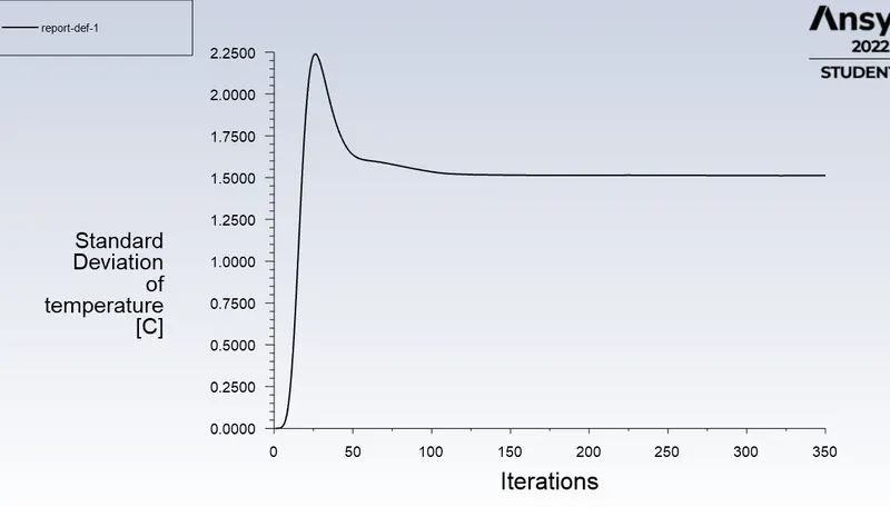
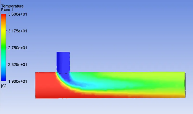
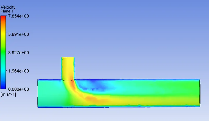
Short pipe
momentum ratio -4
cell count - 22296
Long pipe
momentum ratio -2
cell count - 15727
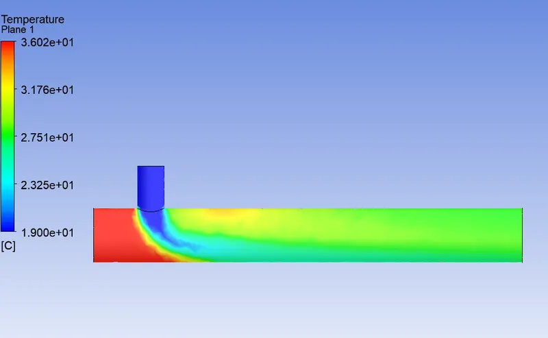
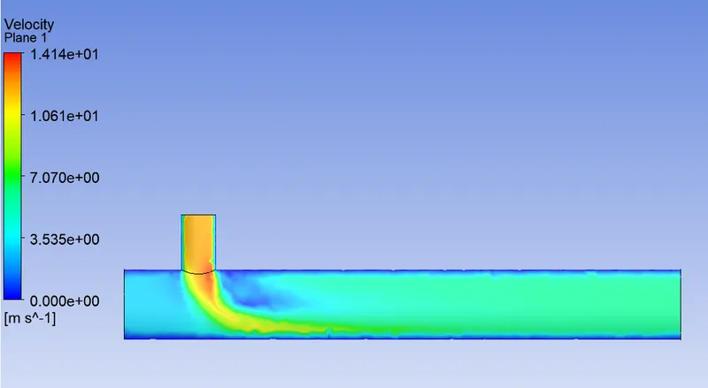
Short pipe
momentum ratio -2
cell count - 15727
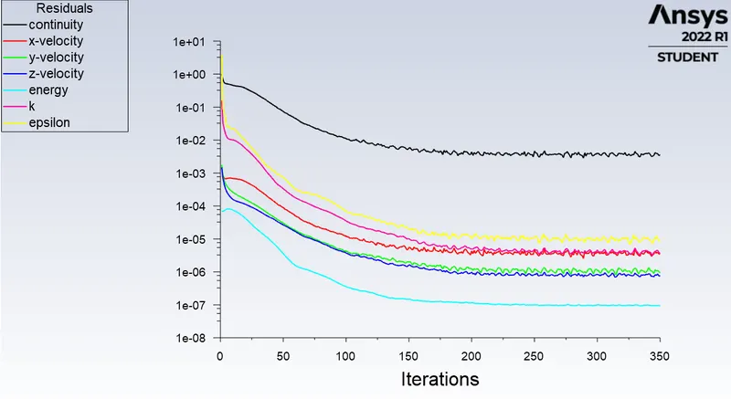
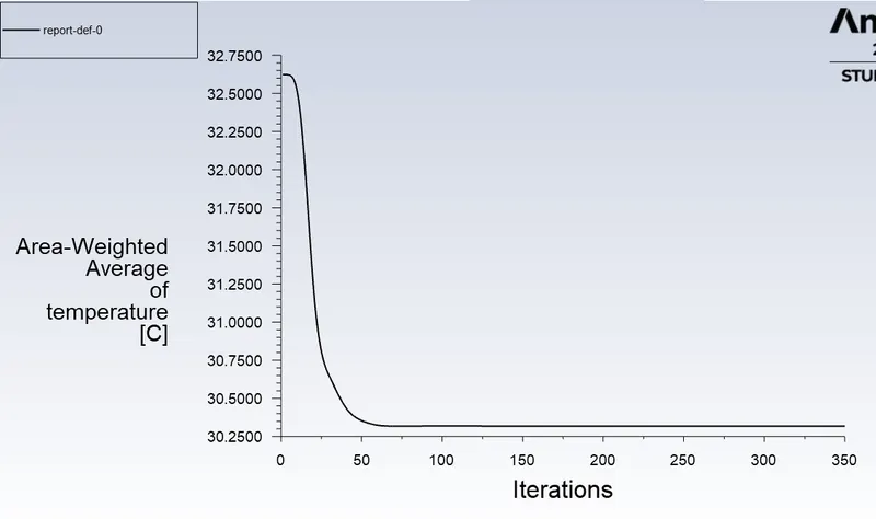
Long pipe
momentum ratio -2
cell count - 56670
Short pipe
momentum ratio -2
cell count - 56670
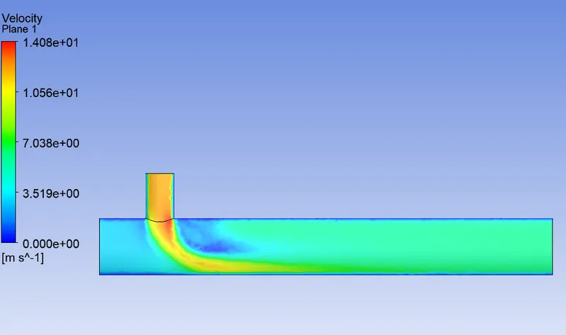
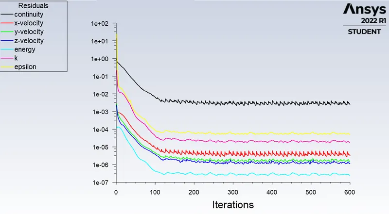
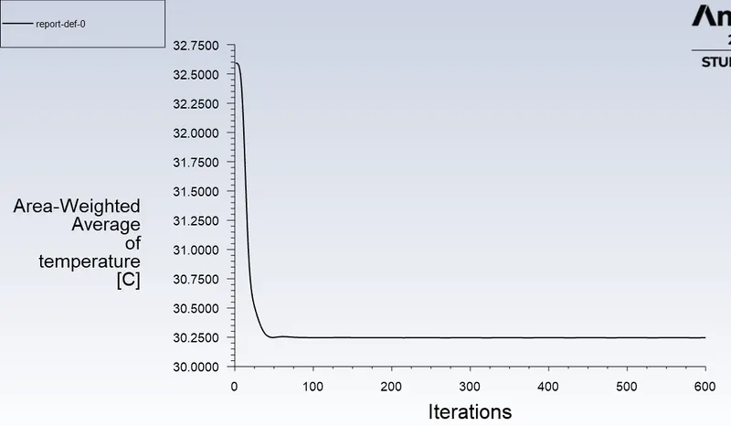
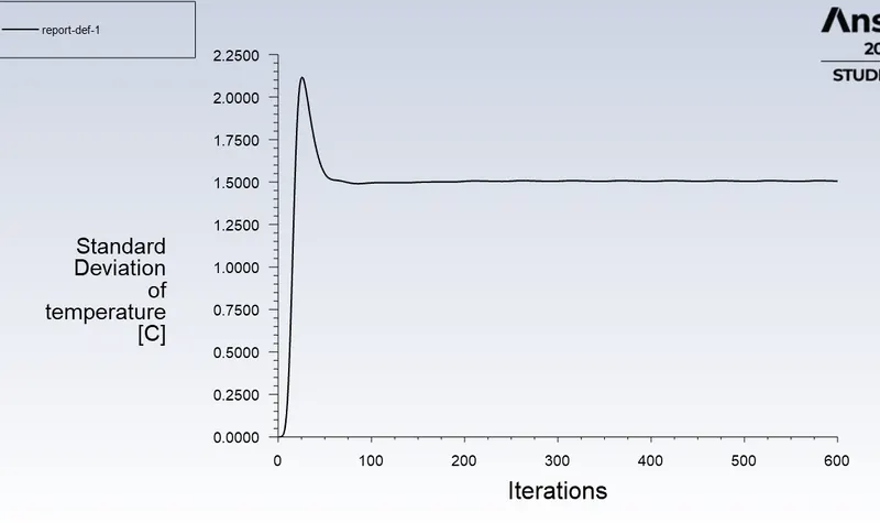
Short pipe
momentum ratio -2
cell count - 44250
| Pipe | momentum ratio | cell count | average temperature outlet(C) |
| short | 2 | 12613 | 30.23 |
| short | 4 | 12613 | 27.55 |
| short | 2 | 22296 | 30.26 |
| short | 4 | 22296 | 27.56 |
| long | 2 | 15727 | 30.261 |
| long | 4 | 15727 | 27.49 |
| long | 2 | 56670 | 30.31 |
| long | 4 | 56670 | 27.53 |