Week 7 - Auto ignition using Cantera
Aim:
To simulate the Auto Ignition Time for Methane under the following conditions, (simulation time = 10 secs)
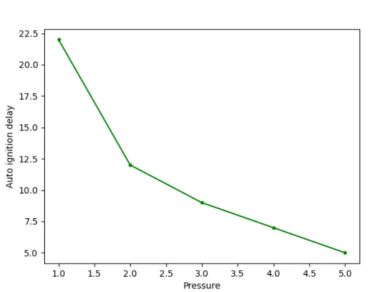
- Plot the variation of Auto Ignition time of Methane with a constant temperature of 1250K and pressure varying from 1 to 5 atm.
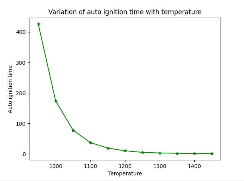
- Plot the variation of Auto Ignition time of Methane with a constant pressure of 5 atm and temperature varying from 950K to 1450K
To print the rate of change of molar concentrations of the given elements "H2O, O2, OH" with respect to the time, (simulation time = 10 secs) and explain the behavior of the graph for 2 cases,
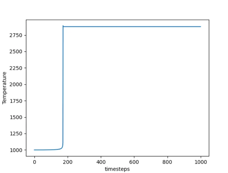
- When Temperature is 1000K and pressure 5 bar
- When Temperature is 500K and pressure 5 bar.
Reactor network:
A Cantera Reactor() represents the simplest form of a chemically reacting system. It corresponds to an extensive thermodynamic control volume VV, in which all state variables are homogeneously distributed. The system is generally unsteady -- that is, all states are functions of time. In particular, transient state changes due to chemical reactions are possible. However, thermodynamic (but not chemical) equilibrium is assumed to be present throughout the reactor at all instants of time.
Reactors can interact with the surrounding environment in multiple ways:
-
Expansion/compression work: By moving the walls of the reactor, its volume can be changed and expansion or compression work can be done by or on the reactor.
-
Heat transfer: An arbitrary heat transfer rate can be defined to cross the boundaries of the reactor.
-
Mass transfer: The reactor can have multiple inlets and outlets. For the inlets, arbitrary states can be defined. Fluid with the current state of the reactor exits the reactor at the outlets.
-
Surface interaction: One or multiple walls can influence the chemical reactions in the reactor. This is not just restricted to catalytic reactions, but mass transfer between the surface and the fluid can also be modeled.
All of these interactions do not have to be constant, but can vary as a function of time or state. For example, heat transfer can be described as a function of the temperature difference between the reactor and the environment, or the wall movement can be modeled depending on the pressure difference. Interactions of the reactor with the environment are defined on one or more walls, inlets, and outlets.
Code:
Case 1:Variation of Auto Ignition time of Methane with a constant temperature of 1250K and pressure varying from 1 to 5 atm.
import sys
import numpy as np
import cantera as ct
import matplotlib.pyplot as plt

gas =ct.Solution('gri30.xml')
P = np.linspace(1,5,5)
T_init=1250
time_start=0.0
time_end=10.0
time_step=1e-3
n=int((time_end-time_start)/time_step)
states_It=[]
time_It=[]

for i in P:
	gas.TPX= T_init,i*101325,{'CH4':1,'O2':2,'N2':7.52}
	T_autoI=0
	t_autoI=0
	time=0
	r=ct.IdealGasReactor(gas)
	sim=ct.ReactorNet([r])
	states=ct.SolutionArray(gas,extra=['time_in_ms','t'])
	print('{:10s} {:10s} {:10s}'.format('t [s]','T [K]','P [Pa]'))

	for j in range(n):
		time+=1e-3
		sim.advance(time)
		states.append(r.thermo.state,time_in_ms=time*1e3,t=time)
		print('{:10.3e} {:10.3f} {:10.3f}'.format(sim.time,r.T,r.thermo.P))
	states_It.append(states.T)

	for i in range(n):
		T_error=states. T[i]- T_init - 400
		if T_error > 0:
			T_autoI=states.T[i]
			t_autoI=states.time_in_ms[i]
			break
	time_It.append(t_autoI)

states_It=np.array(states_It)
for k in range(len(P)):
	plt.plot(states_It[k])
	plt.xlabel('Number of time steps')
	plt.ylabel('Temperature')
	plt.title('Variation of Auto ignition temperature with varying Pressure')
	plt.legend(['1bar','2bar','3bar','4bar','5bar'])

plt.figure(2)
plt.plot(P,time_It,'g.-')
plt.xlabel('Pressure')
plt.ylabel('Auto ignition delay')
plt.show()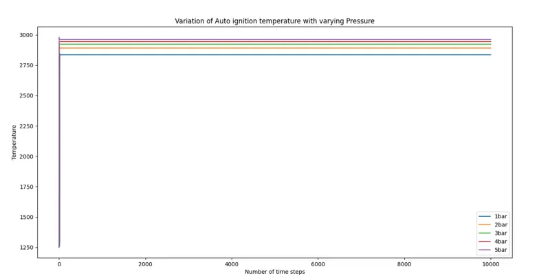
Case 2:Variation of Auto Ignition time of Methane with a constant pressure of 5 atm and temperature varying from 950K to 1450K.
import sys
import numpy as np
import cantera as ct
import matplotlib.pyplot as plt

gas =ct.Solution('gri30.xml')
T= np.linspace(950,1450,11)
P_init=5*101325
time_start=0.0
time_end=10.0
time_step=1e-3
n=int((time_end-time_start)/time_step)
states_It=[]
time_It=[]

for i in T:
    gas.TPX= i,P_init,{'CH4':1,'O2':2,'N2':7.52}
    T_autoI=0
    t_autoI=0
    time=0
    r=ct.IdealGasReactor(gas)
    sim=ct.ReactorNet([r])
    states=ct.SolutionArray(gas,extra=['time_in_ms','t'])
    print('{:10s} {:10s} {:10s}'.format('t [s]','T [K]','P [Pa]'))

    for j in range(n):
        time+=1e-3
        sim.advance(time)
        states.append(r.thermo.state,time_in_ms=time*1e3,t=time)
        print('{:10.3e} {:10.3f} {:10.3f}'.format(sim.time,r.T,r.thermo.P))
    states_It.append(states.T)

    for j in range(n):
        T_error=states.T[j]- i - 400
        if T_error > 0:
            T_autoI=states.T[j]
            t_autoI=states.time_in_ms[j]
            break
    time_It.append(t_autoI)

states_It=np.array(states_It)
for k in range(len(T)):
    plt.plot(states_It[k])
    plt.xlabel('Number of timesteps')
    plt.ylabel('Temperature')
    plt.title('Varaiation of auto ignition temperature with varying inlet temperature ')
    plt.legend(['950K','1000K','1050K','1100k','1150K','1200K','1250K','1300K','1350K','1400K','1450K'])

plt.figure(2)
plt.plot(T,time_It,'g-*')
plt.xlabel('Temperature')
plt.ylabel('Auto ignition time')
plt.title ('Variation of auto ignition time with temperature')
plt.show()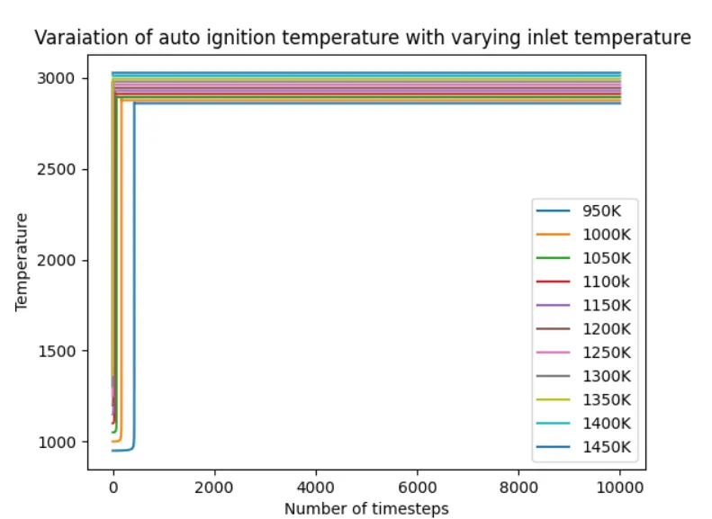
Case 3:The rate of change of molar concentrations of the given elements "H2O, O2, OH" with respect to the time.
import sys
import numpy as np
import cantera as ct
import matplotlib.pyplot as plt

gas =ct.Solution('gri30.xml')
T= np.linspace(950,1450,11)
P_init=5*101325
time_start=0.0
time_end=10.0
time_step=1e-3
n=int((time_end-time_start)/time_step)
states_It=[]
time_It=[]

for i in T:
    gas.TPX= i,P_init,{'CH4':1,'O2':2,'N2':7.52}
    T_autoI=0
    t_autoI=0
    time=0
    r=ct.IdealGasReactor(gas)
    sim=ct.ReactorNet([r])
    states=ct.SolutionArray(gas,extra=['time_in_ms','t'])
    print('{:10s} {:10s} {:10s}'.format('t [s]','T [K]','P [Pa]'))

    for j in range(n):
        time+=1e-3
        sim.advance(time)
        states.append(r.thermo.state,time_in_ms=time*1e3,t=time)
        print('{:10.3e} {:10.3f} {:10.3f}'.format(sim.time,r.T,r.thermo.P))
    states_It.append(states.T)

    for j in range(n):
        T_error=states.T[j]- i - 400
        if T_error > 0:
            T_autoI=states.T[j]
            t_autoI=states.time_in_ms[j]
            break
    time_It.append(t_autoI)

states_It=np.array(states_It)
for k in range(len(T)):
    plt.plot(states_It[k])

plt.figure(2)
plt.plot(T,time_It,'g-*')

plt.figure(3)
plt.subplot(3,1,1)
plt.plot(states.t,states.X[:,gas.species_index('H2O')])
plt.subplot(3,1,2)
plt.plot(states.t,states.X[:,gas.species_index('O2')])
plt.subplot(3,1,3)
plt.plot(states.t,states.X[:,gas.species_index('OH')])
plt.show()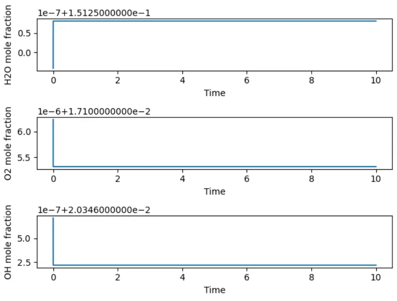
Case 4:When Temperature is 500K and pressure 5 bar
import sys
import numpy as np
import cantera as ct
import matplotlib.pyplot as plt

gas = ct.Solution('gri30.xml')
Pressure= 5*101325
Temperature=[500,1000]
states1=[]


for i in Temperature:
	gas.TPX=500,Pressure,{'CH4':1,'O2':2,'N2':7.52}
	r=ct.IdealGasReactor(gas)
	sim=ct.ReactorNet([r])
	time=0
	states=ct.SolutionArray(gas)

	for i in range(1000):
		time+=1e-3
		sim.advance(time)
		states.append(r.thermo.state)

states1=np.array(states.T)

for k in range(1000):
	plt.plot(states1)
	plt.xlabel('timesteps')
	plt.ylabel('Temperature')
	plt.show()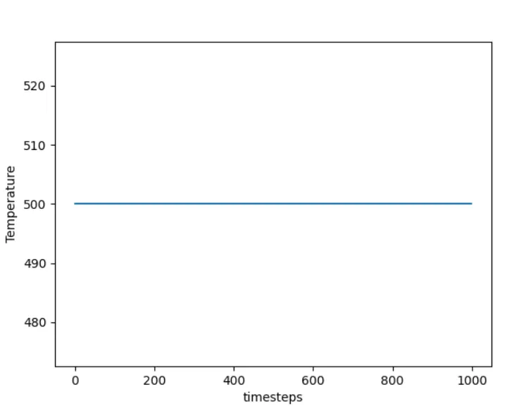
Case 4.2: When Temperature is 1000K and pressure 5 bar
Code explanation:
- At first we import necessary libraries and the initial temperature and pressure are specified.
- We are creating two arrays to store the values of auto ignition temperature and time and the states at each time step
- Then in the for loop we call the reactor network and we find the solution array for the gas.
- Then we advance in simulation using a for loop and append the values of temperature,time in the state.
- Then we find the corresponding temperature and time for the auto ignition delay and store them in the arrays created earlier and plot the results graphically.
- we can use states.X[:,gas.species_index('species')]) to find the mole fraction of species.
Conclusion:
case 1:we can see with increase in pressure ,we find the auto ignition delay decreasing.As pressure increase the temperature.
case 2: As the temperature increases the auto ignition time decreases.This is at high temperature auto ignition takes place at a faster rate.
Case3:We used states.X[:,gas.species_index('species')]) to find the mole fraction of different species.
Case4.1: At 500k the auto ignition doesn't take place as the temperature is low to start the ignition.
case 4.2: At 1000k the auto ignition takes place after a period time in ms.The time delay after which the temperature rises exponentially is called auto ignition delay.