Week 5 - Rayleigh Taylor Instability

Aim:

To perform Rayleigh Taylor instability CFD simulation.

Objectives:

1. What are some practical CFD models that have been based on the mathematical analysis of Rayleigh Taylor waves? In your own words, explain how these mathematical models have been adapted for CFD calculations.
2. Perform the Rayleigh Taylor instability simulation for 2 different mesh sizes with the base mesh being 0.5 mm. Compare the results by showing the animations( Attach them from your google drive). Observe the differences in the animation and explain the effect of mesh size on simulation. Also, explain why a steady-state approach might not be suitable for these types of simulation.[ Choose Air and Water for this simulation]
3. Run one more simulation with water and user-defined material(density = 400 kg/m³, viscosity = 0.001 kg/m-s) for refined mesh.
4. Define the Atwood Number. Find out the Atwood number for both the cases and explain how the variation in Atwood number in the above two cases affects the behavior of the instability.

Practical CFD models that have been based on the mathematical analysis of Rayleigh Taylor waves:

Kelvin Helmholtz instability:

It is a fluid instability occurs due to velocity shear of a single continuous fluid flow or velocity and density difference between two fluids at the interface.It is visible in atmosphere of the planets like the formation of clouds on Earth atmosphere.

Numerically, the Kelvin–Helmholtz instability is simulated in a temporal or a spatial approach. In the temporal approach, the flow is considered in a periodic (cyclic) box "moving" at mean speed (absolute instability). In the spatial approach, simulations mimic a lab experiment with natural inlet and outlet conditions (convective instability).

Richtmyer–Meshkov instability:

The Richtmyer–Meshkov instability (RMI) occurs when two fluids of different density are impulsively accelerated. Normally this is by the passage of a shock wave. The development of the instability begins with small amplitude perturbations which initially grow linearly with time. This is followed by a nonlinear regime with bubbles appearing in the case of a light fluid penetrating a heavy fluid, and with spikes appearing in the case of a heavy fluid penetrating a light fluid. A chaotic regime eventually is reached and the two fluids mix. This instability can be considered the impulsive-acceleration limit of the Rayleigh Taylor instability.

Plateau–Rayleigh instability:

The Plateau–Rayleigh instability, often just called the Rayleigh instability, explains why and how a falling stream of fluid breaks up into smaller packets with the same volume but less surface area. It is related to the Rayleigh-Taylor instability and is part of a greater branch of fluid dynamics concerned with fluid thread breakup. This fluid instability is exploited in the design of a particular type of ink jet technology whereby a jet of liquid is perturbed into a steady stream of droplets.

The driving force of the Plateau–Rayleigh instability is that liquids, by virtue of their surface tensions, tend to minimize their surface area. A considerable amount of work has been done recently on the final pinching profile by attacking it with self- similar solutions.

Rayleigh–Taylor instability:

The Rayleigh–Taylor instability, or RT instability , is an instability of an interface between two fluids of different densities which occurs when the lighter fluid is pushing the heavier fluid. Examples include the behavior of water suspended above oil in the gravity of Earth,mushroom clouds like those from volcanic erruptions and atmospheric nuclear explosions , supernova explosions in which expanding core gas is accelerated into denser shell gas,instabilities in plasma fusion reactors and inertial confinement fusion.

Simulation geometry :

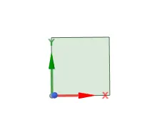
First create a square of 20x20 mm in X-Y plane and use the pull tool to make a surface out of it. Then create a new component and other 20x20mm square on the existing gemetry and again use the pull tool to create surface.

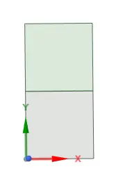
Then use the share topology ,shareprep on the workbench for the conformal meshing of the surfaces.In this simulation the top surface is the water and the bottom surface is air at t=0s.Due to gravitational forces the water comes and the air goes up so there occurs a instability between the layers.

Meshing:

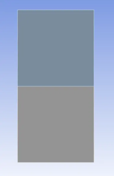
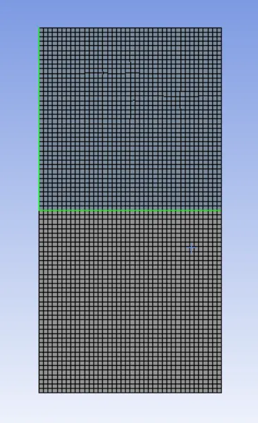
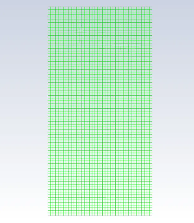
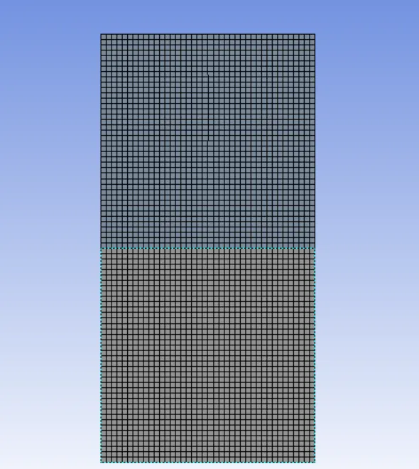
We are going to run the gemetry with two mesh setups ,the normal or baseline mesh setup with 0.5 mm and are asked to run grid independency test on the simulation. As it is not a complicated geometry we only change the element size to run grid dependency.

Simulation Setup:

We use pressure based solver and we use the gravity constrain turned on and specify the value of gravity on the negative axis.We use transient simulation to run simulation with respect to time.

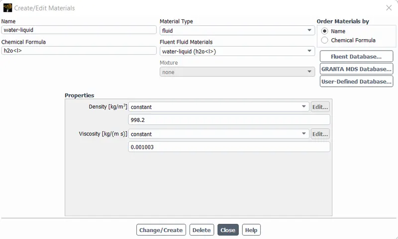
We use laminar flow and add water in the materials from the fluent data base and choose multiphase option and select volume of fluid and set the water and air phases respectively.

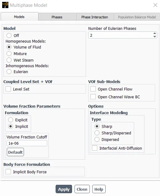
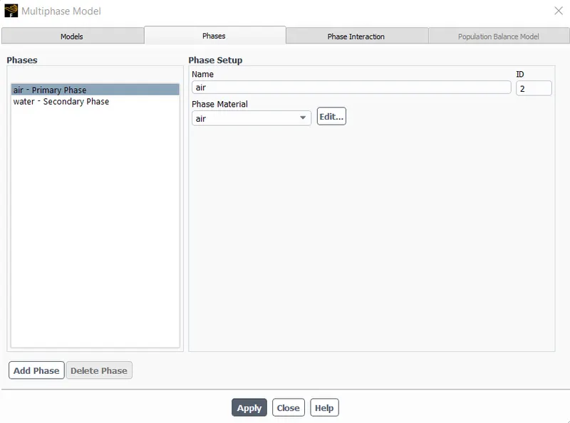
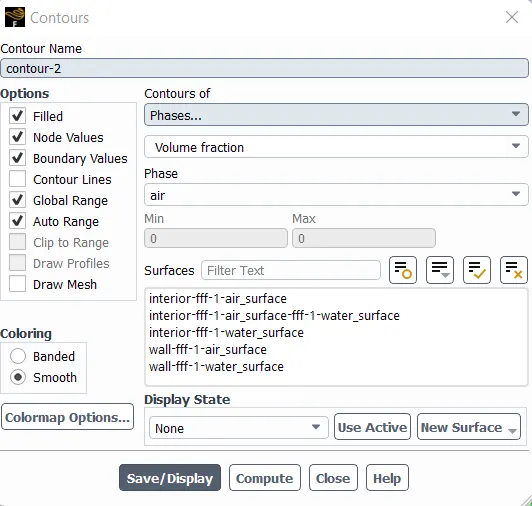
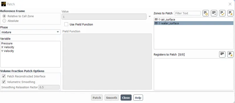
Initialize the solution using standard hybridization.And use the patches and specify the value 1 for water and 0 for air.Add the contour for phases using volume fraction for all the surfaces.

Case 1:

mesh size = 0.05m

step size = 0.025

number of iterations =100

Water and air as the fluids

Mesh:

Residuals:

Volume fraction:

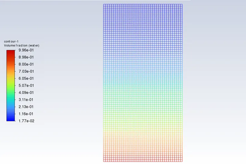
Animation link for this case:

https://drive.google.com/file/d/1h0yTlum2a0PJinHlgvmqmH1hwNhL4WQJ/view?usp=sharing

Case 2:

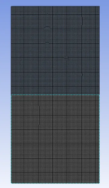
mesh with 0.25mm,

elements = 12800

water and air as fluids

step size =0.025

no.of steps=100

Mesh:

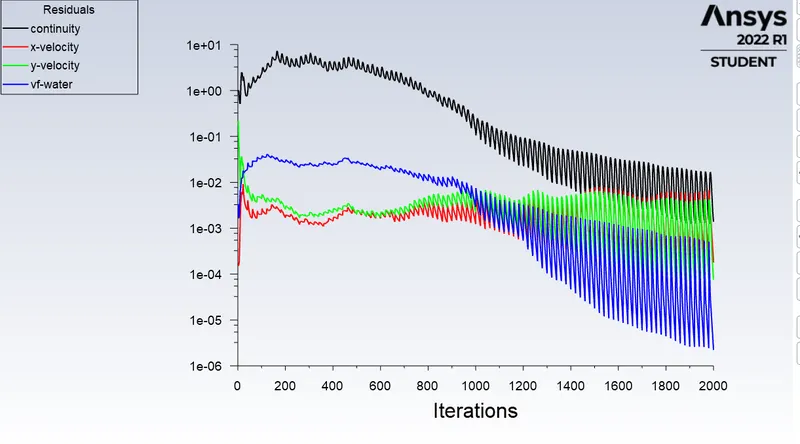
Residuals:

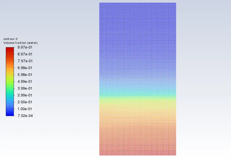
Volume fraction:

Animation for this meshing:

https://drive.google.com/file/d/13m_svaZiIUdb99Tb4hMXG3AharQw7JTT/view?usp=sharing

Case 3:

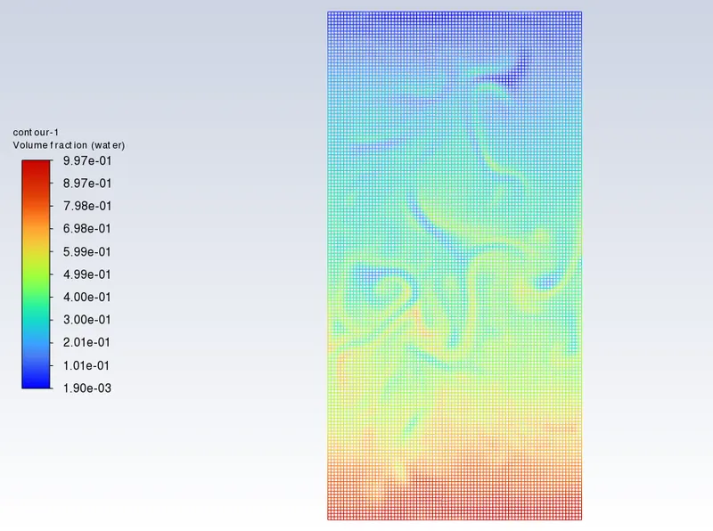
User defined material with density = 400kg/m^3

viscosity = 0.001kg/m-s

mesh =0.25mm

step size =0.025

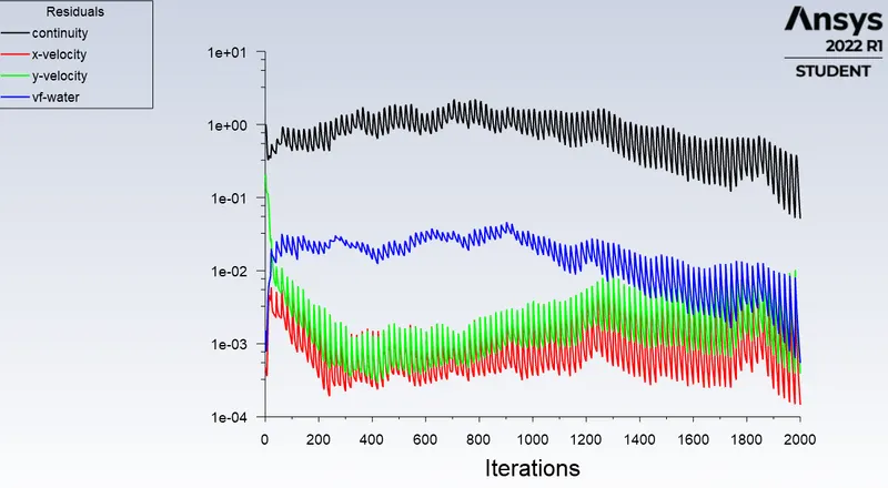
no.of steps=100

Residuals:

Volume fraction:

Atwood number :

The Atwood number (A) is a dimensionless number in fluid dynamics used in the study of hydrodynamic instabilities in density stratified flows. It is a dimensionless density ratio defined as

where

= density of heavier fluid

= density of lighter fluid

Atwood number for case 1:

`rho1= 998.2(kg)/m^3`

`rho2=1.225(kg)/m^3`

A=(998.2- 1.225)/(998.2+1.225) = 0.9975

Atwood number for case 2:

`rho1= 998.2(kg)/m^3`

`rho2=400(kg)/m^3`

A=(998.2-400)/(998.2+400) = 0.4278

Behaviour of Rt instability on Atwood number:

Rt instability evolves in three distinct stages: Linear stability,mushroom head or bubble rising ,Long term evolution due to bubble merging and mixing .for a low Atwood number the mushroom head and bubble rising are relatively similar and the perturbations are linear for a larger time step.but incase of high Atwood number the mushroom and bubble shape is less symmetrical and occurs rapidly at accelerating rate so a non linear growth is seen.

Conclusion:

In this challenge the rayleigh taylor instability ,the lighter fluid (air) pushes the heavier fluid (water ).So we can see the the shock waves being generated at the interference so which the bubbles occurs due the mixing at the interface.

As we refine the mesh the simulation result gets smoother about the irregularities ath the interface.

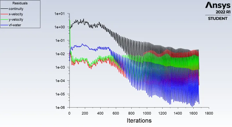
We came across floating point exception in refined mesh case so we used a under relaxation factor for velocity and the momentum and used coupled scheme and used lowest upwind order scheme to get a smoother simulation.

Due to sudden collapse at the interface between the fluid surfaces sudden shocks and irregularities have been formed so we used a transient solver which is time dependent.