Week 7 - Simulation of a 1D Super-sonic nozzle flow simulation using Macormack Method

Objective:

To simulate the isentropic flow through a quasi 1D subsonic-supersonic nozzle by deriving both the conservation and non-conservation forms of the governing equations and sovle them using the MacCormack's technique.

Problem statement:

1. Steady-state distribution of primitive variables inside the nozzle.
2. Time-wise variation of the primitive variables.
3. Variation of Mass flow rate distribution inside the nozzle at different time steps during the time-marching process.
4. Comparison of Normalized mass flow rate distributions of both forms.

MacCormack method:

In computational fluid dynamics the MacCormack method is a widely used discretization scheme for the numerical solution of hyperbolic partial differential equations.

The MacCormack method is a variation of the two-step Lax–Wendroff scheme but is much simpler in application.

The application of MacCormack method to the above equation proceeds in two steps; a predictor step which is followed by a corrector step.

Then the average step is used to find the primitive variables which is the average of predictor and corrector step.

Predictor step uses forward differencing method whereas corrector step uses backward differencing.

- Predictor step

- Corrector step

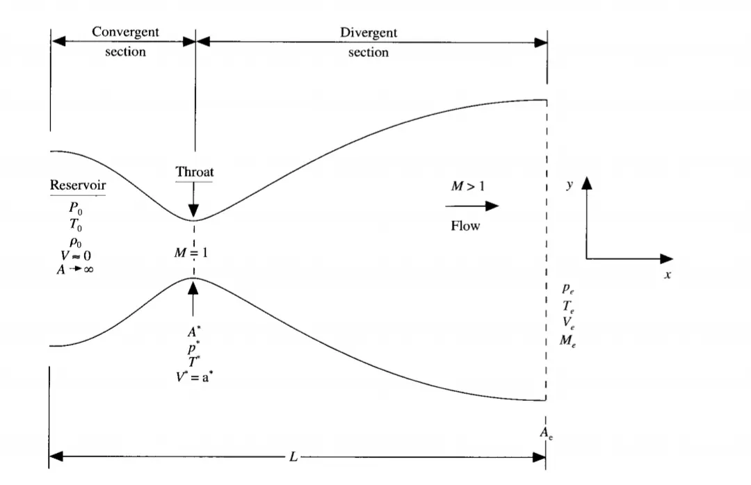
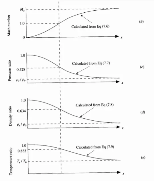
This is the convergent divergent nozzle.the inlet of the nozzle is connected to a tank or reservoir. So the pressure,Temperature velocity are considered to be same as that of the reservoir.

Non conservative form:

Non dimensional quantities:

Temperature - T'=T/`T_0`

Density - `rho'`=`rho/rho_0`

Non dimensional distance - x'=x/L

Area of cross section =A'=A/A*

Non dimensional time t=t/(L/`a_0`) where L/`a_0`is characteristic time scale

Predictor step:

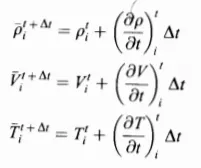
Average step:

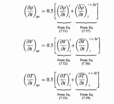
The predictor corrector sequence is repeated at all grid points to obtain density throughout the flow field at time t+dt

we can use the same technique to solve the u,v and T at t+dt

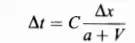
where dt is calculated as

Boundary conditions:

Inflow conditions

`V_1= 2V_2-V_3`

Outflow conditions

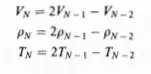
Initial conditions:p

p=1-0.3146*x

T=1-0.2314*x

V=(0.1+1.09*x)T^(1/2)

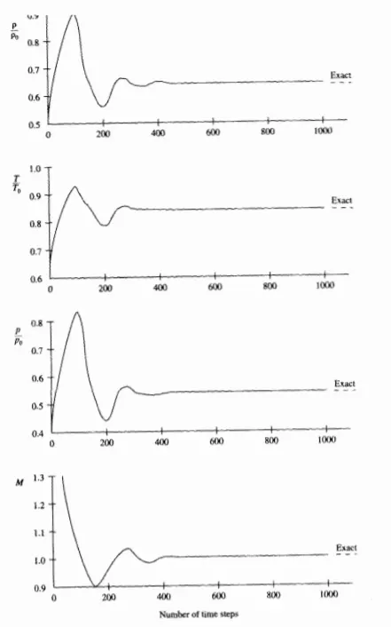
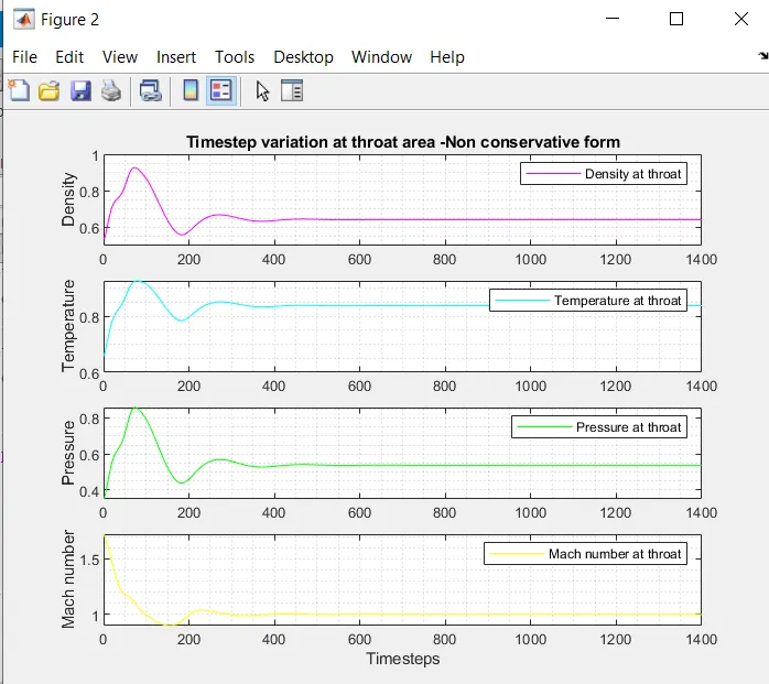
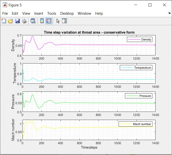
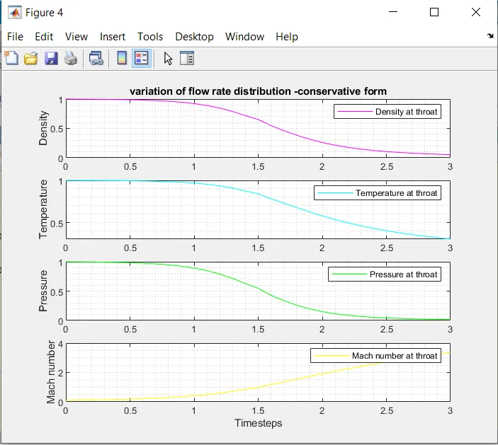
Time step variation graphs at throat area:(Pressure,Temperature,Density and Mach number)

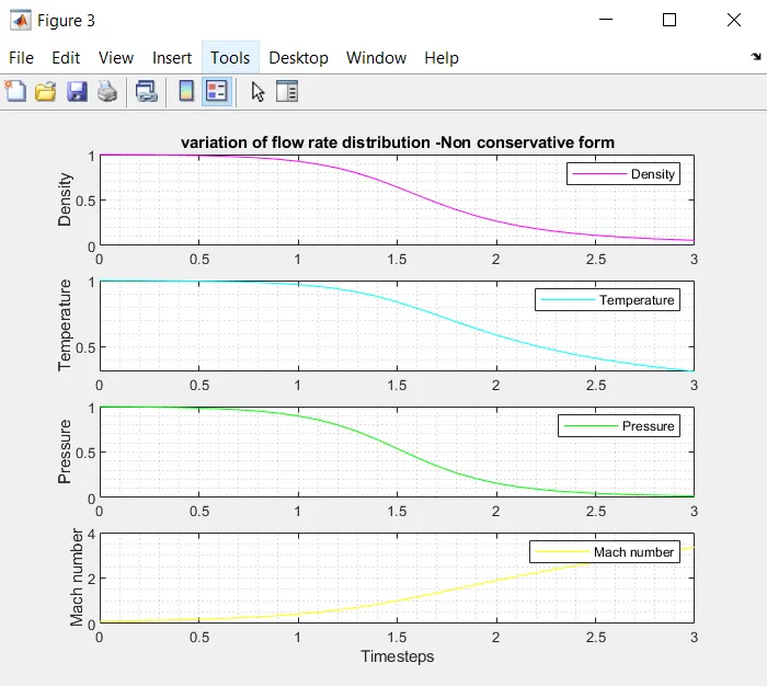
Variation of flow rate distribution:

Main code (MATLAB):

clear all
close all
clc

L=3;%length of nozzle
n=31;%number of grid points
x=linspace(0,L,n);
dx=x(2)-x(1);
nt=1400;
cfl=0.5;
throat=(n-1)/2;
a=1+(2.2*(x-1.5).^2);


%non conservative
[m_nc,M_nc,v,T,p,rho,v_th_nc,p_th_nc,T_th_nc,rho_th_nc,M_th_nc,m_th_nc]=non_conservative(x,dx,n,nt,cfl,a);


%time wise variation of density pressureand temperrature for non conservative
%Density
figure(2)
subplot(4,1,1)
plot(linspace(1,nt,nt),rho_th_nc,'color','m')
ylabel('Density')
legend({'Density at throat'});
% axis([0 1400 0 1.3])
grid minor
title('Timestep variation at throat area -Non conservative form')

%Temperature
subplot(4,1,2)
plot(linspace(1,nt,nt),T_th_nc,'color','c')
ylabel('Temperature')
legend({'Temperature at throat'});
% axis([0 1400 0.6 1])
grid minor
%pressure
subplot(4,1,3)
plot(linspace(1,nt,nt),p_th_nc,'color','g')
ylabel('Pressure')
legend({'Pressure at throat'});
% axis([0 1400 0.4 1.1])
grid minor
%mach number
subplot(4,1,4)
plot(linspace(1,nt,nt),M_th_nc,'color','y')
xlabel('Timesteps')
ylabel('Mach number')
legend({'Mach number at throat'});
% axis([0 1400 0.6 1.4])
grid minor

figure(3)
subplot(4,1,1)
plot(x,rho,'color','m')
ylabel('Density')
legend({'Density'});
% axis([0 3 0 1])
grid minor
title('variation of flow rate distribution -Non conservative form')

subplot(4,1,2)
plot(x,T,'color','c')
ylabel('Temperature')
legend({'Temperature'});
% axis([0 3 0 1])
grid minor

%pressure
subplot(4,1,3)
plot(x,p,'color','g')
ylabel('Pressure')
legend({'Pressure'});
% axis([0 3 0 1])
grid minor

subplot(4,1,4)
plot(x,M_nc,'color','y')
xlabel('Timesteps')
ylabel('Mach number')
legend({'Mach number'});
% axis([0 3 0 4])
grid minor
%%


% 
% %Conservative form
% 
[m_c,M_c,v_c,T_c,p_c,rho_c,v_th_c,p_th_c,T_th_c,rho_th_c,M_th_c,m_th_c]=conservative(x,dx,n,nt,cfl,a);


%Density
figure(4)
subplot(4,1,1)
plot(x,rho_c,'color','m')
ylabel('Density')
legend({'Density at throat'});
% axis([0 1400 0 1.3])
grid minor
title('Timestep variation at throat area -conservative form')

%Temperature
subplot(4,1,2)
plot(x,T_c,'color','c')
ylabel('Temperature')
legend({'Temperature at throat'});
% axis([0 1400 0.6 1])
grid minor
%pressure
subplot(4,1,3)
plot(x,p_c,'color','g')
ylabel('Pressure')
legend({'Pressure at throat'});
% axis([0 1400 0.4 1.1])
grid minor
%mach number
subplot(4,1,4)
plot(x,M_c,'color','y')
xlabel('Timesteps')
ylabel('Mach number')
legend({'Mach number at throat'});
% axis([0 1400 0.6 1.4])
grid minor
% 
figure(5)
subplot(4,1,1)
plot(linspace(1,nt,nt),rho_th_c,'color','m')
ylabel('Density')
legend({'Density'});
% axis([0 3 0 1])
grid minor
title('Varistion of flow rate distribution - conservative form')
% 
subplot(4,1,2)
plot(linspace(1,nt,nt),T_th_c,'color','c')
ylabel('Temperature')
legend({'Temperature'});
% axis([0 3 0 1])
grid minor
% 
%pressure
subplot(4,1,3)
plot(linspace(1,nt,nt),p_th_c,'color','g')
ylabel('Pressure')
legend({'Pressure'});
% axis([0 3 0 1])
grid minor
% 
subplot(4,1,4)
plot(linspace(1,nt,nt),M_th_c,'color','y')
xlabel('Timesteps')
ylabel('Mach number')
legend({'Mach number'});
% axis([0 3 0 4])
grid minor

%comparison Mass flow rate of both forms
figure(8)
plot(x,m_nc,'linewidth',1.25)
hold on
plot(x,m_c,'linewidth',1.25)
grid on

legend('Non-Conservative','Conservative')
xlabel('Length of Domain')
ylabel('Mass flow rate')
title('comparison of both mass flow rates')

Non conservative form code:

%non conservative form
function [m_nc,M_nc,v,T,p,rho,v_th,p_th,T_th,rho_th,M_th,m_th]=non_conservative(x,dx,n,nt,cfl,a)
%initial conditions

rho=1-(0.3146*x);
T=1-0.2314*x;
v=(0.1+1.09.*x).*T.^0.5;
M_nc=v./(T.^0.5);
m_nc=rho.*a.*v;
p=rho.*T;
gamma=1.4;
th=find(a==1);

for k=1:nt
    for i=1:n
        dt=min(cfl.*(dx./(sqrt(T)+v)));
    end
    
    rho_old=rho;
    T_old=T;
    v_old=v;
    %predictor step
    for j=2:n-1
        %simplyfying the equations
        dv_dx=(v(j+1)-v(j))/dx;
        drho_dx=(rho(j+1)-rho(j))/dx;
        dT_dx=(T(j+1)-T(j))/dx;
        dlog_a_dx=(log(a(j+1))-log(a(j)))/dx;
        
        dhorho_dt_p(j)= -rho(j)*(dv_dx) - (rho(j)*v(j)*dlog_a_dx)-v(j)*drho_dx;%continiuity equation
        dhov_dt_p(j)= -v(j)*(dv_dx)-(1/gamma)*((dT_dx+(T(j)/rho(j)*drho_dx)));%momentum equation
        dhoT_dt_p(j)=-v(j)*(dT_dx)-(gamma-1)*T(j)*(dv_dx + (v(j)*dlog_a_dx));%energy equation
        
        
        %solution update
        rho(j)=rho(j)+dhorho_dt_p(j)*dt;
        v(j)=v(j)+dhov_dt_p(j)*dt;
        T(j)=T(j)+dhoT_dt_p(j)*dt;
    end
    %corrector step
     for j=2:n-1
        %simplyfying the equations
        dv_dx=(v(j)-v(j-1))/dx;
        drho_dx=(rho(j)-rho(j-1))/dx;
        dT_dx=(T(j)-T(j-1))/dx;
        dlog_a_dx=(log(a(j))-log(a(j-1)))/dx;
        
        
        dhorho_dt_c(j)= -rho(j)*(dv_dx) - (rho(j)*v(j)*dlog_a_dx)-v(j)*drho_dx;%continiuity equation
        dhov_dt_c(j)= -v(j)*(dv_dx)-(1/gamma)*((dT_dx+(T(j)/rho(j)*drho_dx)));%momentum equation
        dhoT_dt_c(j)=-v(j)*(dT_dx)-(gamma-1)*T(j)*(dv_dx + (v(j)*dlog_a_dx));%energy equation
    
        %solution update
        rho(j)=rho(j)+dhorho_dt_c(j)*dt;
        v(j)=v(j)+dhov_dt_c(j)*dt;
        T(j)=T(j)+dhoT_dt_c(j)*dt;
     end
     %average time derivative
     dhorho_dt=0.5.*(dhorho_dt_p+dhorho_dt_c);
     dhov_dt=0.5.*(dhov_dt_p+dhov_dt_c);
     dhoT_dt=0.5.*(dhoT_dt_p+dhoT_dt_c);
     
     %final solution update
     for i=2:n-1
         rho(i)=rho_old(i)+dhorho_dt(i)*dt;
         v(i)=v_old(i)+dhov_dt(i)*dt;
         T(i)=T_old(i)+dhoT_dt(i)*dt;
     end
     %Applying the boundary conditions
     v(1)=2*v(2)-v(3);
     v(n)=2*v(n-1)-v(n-2);
     T(n)=2*T(n-1)-T(n-2);
     rho(n)=2*rho(n-1)-rho(n-2);
     
     %defining the values of pressure,mach number and mass flow rate
 M_nc=v./(T.^0.5);
m_nc=rho.*a.*v;
p=rho.*T;

rho_th(k)=rho(th);
v_th(k)=v(th);
T_th(k)=T(th);
M_th(k)=M_nc(th);
m_th(k)=m_nc(th);
p_th(k)=p(th);
figure(6)
if k==50
    plot(x,m_nc,'linewidth',1.25);
    hold on
elseif k==100
     plot(x,m_nc,'linewidth',1.25);
    hold on
    elseif k==200
     plot(x,m_nc,'linewidth',1.25);
    hold on
    elseif k==400
     plot(x,m_nc,'linewidth',1.25);
    hold on
    elseif k==800
     plot(x,m_nc,'linewidth',1.25);
    hold off
end
% labelling
title('Mass flow rate at different time rates');
xlabel('Distance');
ylabel('Mass flow rate');
legend({'50^t^h timestep','100^t^h timestep','200^t^h timestep','400^t^h timestep','800^t^h timestep'});
axis([0 3 0 2])
grid on
end

Conservative form:

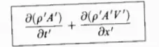- Continuity equation

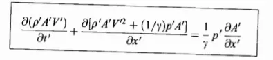- Momentum equation

- Energy equation

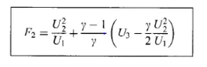
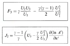
the equations for quasi one dimensional flow can be expressed in a generic form so let us define the elements of the solution vector U and flux vector F and source terms as follows

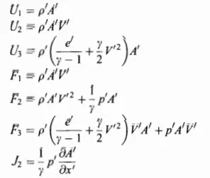
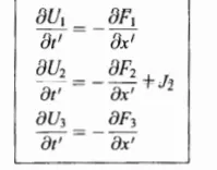
where U is the solution term F is the flux term and J2 is the source term

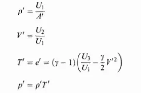
In conservative form we can directly use or find the primitive variables so we use solution vectors so we decode the solution vector to get the primitive variables

Expressing flux terms and source terms in Solution vectors

`F_1 = U_2`

Boundary conditions:

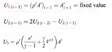
Inlet boundary conditions:

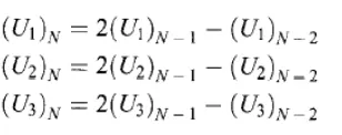
Outlet boundary conditions

Initial conditions:

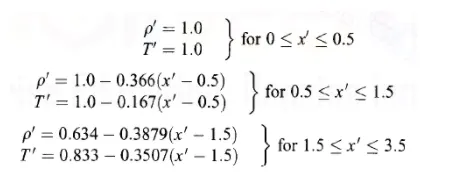
Calculate time step as same as the non conservative method

Conservative form code

%conservative method
function[m_c,M_c,v_c,T_c,p_c,rho_c,v_th_c,p_th_c,T_th_c,rho_th_c,M_th_c,m_th_c]=conservative(x,dx,n,nt,cfl,a)
gamma = 1.4;
for i=1:n
    if(x(i)>=0 && x(i)<=0.5)
        rho_c(i)=1;
        T_c(i)=1;
    elseif(x(i)>=0.5&&x(i)<=1.5)
        rho_c(i)=1-0.366*(x(i)-0.5);
        T_c(i)=1-0.167*(x(i)-0.5);
    elseif(x(i)>=1.5&&x(i)<=3)
        rho_c(i)=0.634-0.3879*(x(i)-1.5);
        T_c(i)=0.833-0.3507*(x(i)-1.5);
    end
end
%Area and throat profiles
a=1+2.2*(x-1.5).^2;
throat=find(a==1);
%initial profile
v_c=0.59./(rho_c.*a);
p_c=rho_c.*T_c;
%calculate initial solution vectors
u1=rho_c.*a;
u2=rho_c.*a.*v_c;
u3=rho_c.*a.*(T_c./(gamma-1))+((gamma/2).*v_c.^2);
%outer loop
for k=1:nt
    dt=min(cfl.*dx./(sqrt(T_c)+v_c));
    %saving a copy of old values
    u1_old=u1;
    u2_old=u2;
    u3_old=u3;
%calculating flux vector
f1=u2;
f2=((u2.^2)./u1)+((gamma-1)/gamma)*(u3-(gamma/2)*((u2.^2)./u1));
f3=((gamma*u2.*u3)./u1)-(gamma*(gamma-1)*((u2.^3)./(2*u1.^2)));


%predictor method
for j=2:n-1
    %calculating source term
    J2(j)=(1/gamma)*rho_c(j)*T_c(j)*((a(j+1)-a(j))/dx);
    
    %continuity equation
    du1_dt_p(j)=-((f1(j+1)-f1(j))/dx);
    %momentum equation
    du2_dt_p(j)=-((f2(j+1)-f2(j))/dx)+J2(j);
    %energy equation
    du3_dt_p(j)=-((f3(j+1)-f3(j))/dx);
    
    %updating new values
    u1(j)=u1(j)+du1_dt_p(j)*dt;
    u2(j)=u2(j)+du2_dt_p(j)*dt;
    u3(j)=u3(j)+du3_dt_p(j)*dt;
end
%updating flux vectors
f1=u2;
f2=((u2.^2)./u1)+((gamma-1)/gamma)*(u3-((gamma*0.5*(u2.^2))./(u1)));
f3=((gamma*u2.*u3)./u1)-((gamma*0.5*(gamma-1)*(u2.^3))./(u1.^2));
  
%corecctor method
for j=2:n-1
    %updating the source term
     J2(j)=(1/gamma)*rho_c(j)*T_c(j)*((a(j)-a(j-1))/dx);
    
    %continuity equation
    du1_dt_c(j)=-((f1(j)-f1(j-1))/dx);
    %momentum equation
    du2_dt_c(j)=-((f2(j)-f2(j-1))/dx)+J2(j);
    %energy equation
    du3_dt_c(j)=-((f3(j)-f3(j-1))/dx);
    
end
%compute average time derivative
du1_dt=0.5*(du1_dt_p+ du1_dt_c);
du2_dt=0.5*(du2_dt_p+du2_dt_c);
du3_dt=0.5*(du3_dt_p+du3_dt_c);
%final solution update
for i=2:n-1
    u1(i)=u1_old(i)+du1_dt(i)*dt;
    u2(i)=u2_old(i)+du2_dt(i)*dt;
    u3(i)=u3_old(i)+du3_dt(i)*dt;
end

%applying boundary conditions
%at inlet
u1(1)=rho_c(1)*a(1);
u2(1)=2*u2(2)-u2(3);
v_c(1)=u2(1)./u1(1);
u3(1)=u1(1)*((T_c(1)/(gamma-1))+((gamma/2)*(v_c(1)).^2));
%at outlet
u1(n)=2*u1(n-1)-u1(n-2);
u2(n)=2*u2(n-1)-u2(n-2);
u3(n)=2*u3(n-1)-u3(n-2);
%final primitive values update
rho_c=u1./a;
v_c=u2./u1;
T_c=(gamma-1)*((u3./u1-(gamma/2)*(v_c).^2));
%defining mass flow rate,pressure and mach number
m_c=rho_c.*a.*v_c;
p_c=rho_c.*T_c;
M_c=(v_c./sqrt(T_c));
%calculating variables at throat section
rho_th_c(k)=rho_c(throat);
T_th_c(k)=T_c(throat);
v_th_c(k)=v_c(throat);
m_th_c(k)=m_c(throat);
p_th_c(k)=p_c(throat);
M_th_c(k)=M_c(throat);

figure(7)
if k==50
    plot(x,m_c,'m','linewidth',1.25);
    hold on
elseif k==100
    plot(x,m_c,'c','linewidth',1.25);
    hold on
elseif k==200
    plot(x,m_c,'g','linewidth',1.25);
    hold on
elseif k==400
    plot(x,m_c,'y','linewidth',1.25);
    hold on
elseif k==800
    plot(x,m_c,'k','linewidth',1.25);
    hold on
end
%labelling
title('Mass flow rates at different time steps- conservative form')
xlabel('Distance')
ylabel('Mass flow rate')
legend({'50^t^h timestep','100^t^h timestep','200^t^h timestep','400^t^h timestep','800^t^h timestep'})
axis([0 3 0.4 1])
grid on
end
end

Explanation of the code:

1.The domain length , grid points ,mesh and cfl values are specified.To determine the initial profile of Temperature ,density,velocity the for loop is used inputing the known conditions.

2.A function is created for non conservative form the time elapsed is stored, the initial values of throat,area ,pressure,density temperature values are calculated using the formulas.

3.The outer time loop is computed to calculate all the grid points for various formulas inside the loop and time step dt value is claculated.

4.Then Maccormack method is used to solve the numerical solution of the governing equation such as continuity ,momentum and energy equation,The predictor ,the corrector step and the average step is calculated and solved .

5.Then final solution update takes place and the boundary conditions are specified at inlet and outlet condition and calculating the primitive variables at throat section and plotting the mass flow rates at diffferent time steps.

6.Then a function for conservative form is created similarlly all the initial conditions are specified in the for loop,In order to simplify and avoid errors,equation is splitted into solution vectors(U) ,flux terms(F) and source terms(J).

7.Then the flux terms and source terms are converted to solution vectors and solved to get the primitive values as same as in the non conservative method and the boundary conditions are specified and used for calculating the Mass flow rate ,Mach number,Pressure and also calculate the values at throat section.

8.The time wise variation and variation of flow rateof Pressure,Mach number,Temperature is plotted in the main code.

Results and conclusion:

Time step variation of primitive variable at throat area

Non-Conservative form:

Conservative form:

Observation:

From the above plots we can conclude that the initial variations observed in non conservaytive form for a certain period of time makes it consume higher amount of time to achieve stable solution when compared to conseravtive form.

Variation of Flow rate distribution:

Non -Conservative:

Conservative form:

Observation:

From the above plots we can see the variation of flow rate distribution is ame for both the forms at each timesteps.

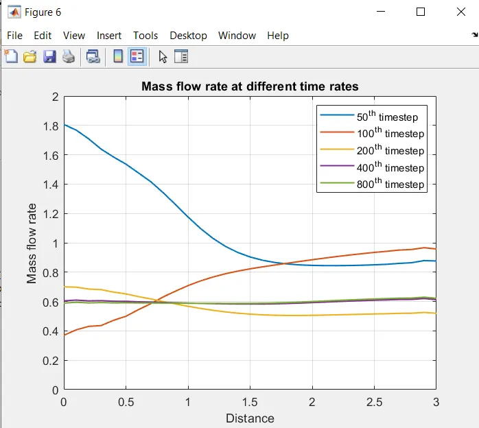
Mass flow rates at different time steps:

Non -Conservative form:

Conservative form:

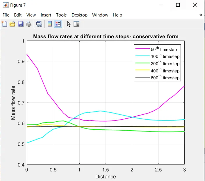
Observation:

From the above plots we can see that the Mass flow rate at different time steps oscillates however after the 400th time steps for both the forms the solution becomes stable and constant value.

Comparison plot of Normalised Mass flow rate of both Non conservative and conservative method:

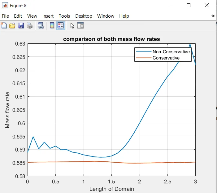
Observation:

When comparing the mass flow rate at different time steps both forms are moreover similar,but the non conservative form solution oscilattes more than the Conservative form.by this we can conclude that conservative formattains stable solution in lesser number of iterations.

Grid dependence test:(Comparison of solutions after 1400 steps)

Grid points	Density	Mach number	Temperature	Velocity	Time elapsed
n=31(conservative)	0.6516	0.9795	0.8406	0.8981	120
n=31(non-conservative)	0.6421	0.9995	0.8380	0.9150	114
n=61(conservative)	0.6383	0.9992	0.8351	0.9132	122.955
n=61(non-conservative)	0.6394	0.9997	0.8362	0.9142	127.34

Observation:

Grid dependence is an important factor to determine whether the problem can be solved faster .So we have increased the grid points from 31 to 61 and tabulated the primitive variables above.

It is clear from the above table that the values are almost same along the primitive variables for both forms even when the grid point is changed from 31 to 61 showing that it doesn't get affected by the increased of grid points.

As we increase the number of grid points we can see that the value approaches very close to the analytical solution but increases the runtime of the program.

The conservative form provide accurate results for the flux quantities whereas the non conservative form provides accurate result for the primitive variables.

Conclusion:

Ultimately from the above results we can conclude that conservative form converges slightly faster than the Non conservation form offering stable solution through simulation.