Week 5.1 - Mid term project - Solving the steady and unsteady 2D heat conduction problem
Objective:
To solve the 2D heat conduction equation by using the point iterative techniques such ad Jacobi,Gauss seidel and successive over relaxation method for implicit and explicit svhemes in MATLAB.
Theory:
The heat conduction equation is a partial differential equation that describes the distribution of heat (or the temperature field) in a given body over time.
For a function u(x,y,z,t) of three spatial derivatives and t of time derivative ,the heat conduction equation is
`delu`/`delt`=`alpha`((`del^2u`/`delx^2`)+(`del^2u`/`delx^2`)+(`del^2u`/`delx^2`))
where `alpha` is diffusivity of the medium.
Types of heat conduction schemes
Steady state heat conduction
Unsteady/Transient heat conduction
Steady-state conduction is the form of conduction that happens when the temperature difference driving the conduction are constant, so that (after an equilibration time), the spatial distribution of temperatures (temperature field) in the conducting object does not change any further.
In unsteady heat conduction the temperature changes with time.
Implicit scheme - Steady state conduction
Steady state equation discretization
In steady state equation the heat entering is equal to heat coming out.
(`del^2u`/`delx^2`)+(`del^2u`/`dely^2`)=0
By discretizing the above equation we get
`T_p`=1/k*((`T_l+T_r`/dx^2)+(`T_T++T_B`/dy^2))
where K=2*((dx^2+dy^2)/(dx^2*dy^2))
If we solve the equation further
`T_p`=(0.5/(dx^2+dy^2))*(dy^2*(T(i-1,j)+T_old(i+1,j))+dx^2*(T(i,j-1)+T_old(i,j+1)))
Steady state equation using implicit scheme using jacobi iteration method:
%steady state equation implicit scheme using jacobi iteration method
clear all
close all
clc
%Solving the steady state 2D heat conduction (Jacobi method)
%Input parameters
nx=10;
ny=10;
x=linspace(0,1,nx);
y=linspace(0,1,ny);
dx=x(2)-x(1);
dy=dx;
error=9e9;
tol=1e-4;
%defining boundary conditions
left_boundary=400;
right_boundary=800;
top_boundary=600;
bottom_boundary=900;

T=300*ones(nx,ny);
%applying the boundary conditions
T(2:ny-1,1)=left_boundary;
T(1,2:nx-1)=top_boundary;
T(ny,2:nx-1)=bottom_boundary;
T(2:ny-1,nx)=right_boundary;
%calculating average values at the corners
T(1,1)=(left_boundary+top_boundary)/2;
T(nx,ny)=(right_boundary+bottom_boundary)/2;
T(1,ny)=(top_boundary+right_boundary)/2;
T(nx,1)=(left_boundary+top_boundary)/2;
%Assigning original values to T
T_initial=T;
T_old=T;

jacobi_iteration=1;
while(error>tol)
    for i=2:nx-1
        for j=2:ny-1
            T(i,j)=(0.5/(dx^2+dy^2))*(dy^2*(T_old(i-1,j)+T_old(i+1,j))+dx^2*(T_old(i,j-1)+T_old(i,j+1)));
        end
    end
    error=max(max(abs(T_old-T)));
    T_old=T;
    jacobi_iteration=jacobi_iteration+1;
end


figure(1)
contourf(x,y,T)
clabel(contourf(x,y,T))
colorbar
colormap
colormap(jet)
set(gca,'ydir','reverse')
title(sprintf('No of jacobi iterations=%d',jacobi_iteration));
xlabel('X-axis')
ylabel('Y-axis')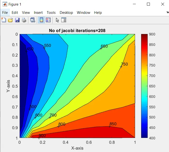
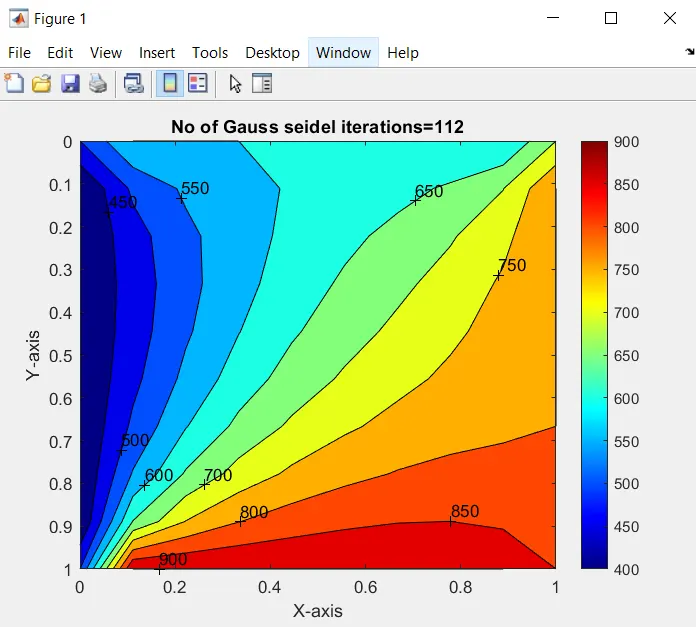
Steady state equation using implicit scheme using Gauss seidel iteration method:
clear all
close all
clc
%Solving the steady state 2D heat conduction (Jacobi method)
%Input parameters
nx=10;
ny=10;
x=linspace(0,1,nx);
y=linspace(0,1,ny);
dx=x(2)-x(1);
dy=dx;
error=9e9;
tol=1e-4;
%defining boundary conditions
left_boundary=400;
right_boundary=800;
top_boundary=600;
bottom_boundary=900;

T=300*ones(nx,ny);
%applying the boundary conditions
T(2:ny-1,1)=left_boundary;
T(1,2:nx-1)=top_boundary;
T(ny,2:nx-1)=bottom_boundary;
T(2:ny-1,nx)=right_boundary;
%calculating average values at the corners
T(1,1)=(left_boundary+top_boundary)/2;
T(nx,ny)=(right_boundary+bottom_boundary)/2;
T(1,ny)=(top_boundary+right_boundary)/2;
T(nx,1)=(left_boundary+top_boundary)/2;
%Assigning original values to T
T_initial=T;
T_old=T;
Gauss_siedel_iteration=1;
while(error>tol)
    for i=2:nx-1
        for j=2:ny-1
            T(i,j)=(0.5/(dx^2+dy^2))*(dy^2*(T(i-1,j)+T_old(i+1,j))+dx^2*(T(i,j-1)+T_old(i,j+1)));
        end
    end
    error=max(max(abs(T_old-T)));
    T_old=T;
    Gauss_siedel_iteration=Gauss_siedel_iteration+1;
end


figure(1)
contourf(x,y,T)
clabel(contourf(x,y,T))
colorbar
colormap
colormap(jet)
set(gca,'ydir','reverse')
title(sprintf('No of Gauss seidel iterations=%d',Gauss_siedel_iteration));
xlabel('X-axis')
ylabel('Y-axis')
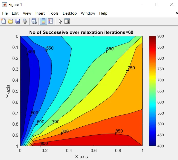
Steady state equation using implicit scheme using Successive over relaxation iteration method:
clear all
close all
clc
%Solving the steady state 2D heat conduction (Jacobi method)
%Input parameters
nx=10;
ny=10;
x=linspace(0,1,nx);
y=linspace(0,1,ny);
dx=x(2)-x(1);
dy=dx;
error=9e9;
tol=1e-4;
omega=1.3;
%defining boundary conditions
left_boundary=400;
right_boundary=800;
top_boundary=600;
bottom_boundary=900;

T=300*ones(nx,ny);
%applying the boundary conditions
T(2:ny-1,1)=left_boundary;
T(1,2:nx-1)=top_boundary;
T(ny,2:nx-1)=bottom_boundary;
T(2:ny-1,nx)=right_boundary;
%calculating average values at the corners
T(1,1)=(left_boundary+top_boundary)/2;
T(nx,ny)=(right_boundary+bottom_boundary)/2;
T(1,ny)=(top_boundary+right_boundary)/2;
T(nx,1)=(left_boundary+top_boundary)/2;
%Assigning original values to T
T_initial=T;
T_old=T;
Successive_over_relaxation_iteration=1;
while(error>tol)
    for i=2:nx-1
        for j=2:ny-1
            T(i,j)=omega*((0.5/(dx^2+dy^2))*(dy^2*(T(i-1,j)+T_old(i+1,j))+dx^2*(T(i,j-1)+T_old(i,j+1))))+(1-omega)*T_old(i,j);
        end
    end
    error=max(max(abs(T_old-T)));
    T_old=T;
    Successive_over_relaxation_iteration=Successive_over_relaxation_iteration+1;
end


figure(1)
contourf(x,y,T)
clabel(contourf(x,y,T))
colorbar
colormap
colormap(jet)
set(gca,'ydir','reverse')
title(sprintf('No of Successive over relaxation iterations=%d',Successive_over_relaxation_iteration));
xlabel('X-axis')
ylabel('Y-axis')
Detailed explanation of the code for steady state implicit scheme:
1.The initial conditions and the grid size and the square area is created .
2. The boundary conditions are of the temperature are specified respectively.
3.the corner values of the matrix are calculated accordingly to boundary conditions specified.
4.T_old and T_initial are assigned with the values of T initiallly and time loop is created for x derivative and y derivative,the omega value is multiplied for the SOr method alone.
5. The governing equation is written and the error value is calculated and the T_old value is updated for the next iteration,and continues till the error value is less than tolerance value
6.Plotting the result in colormap.
Implicit scheme Unsteady state conduction:
`delT`/`delt`=`alpha`*(`del^2T`/`delx^2`)+(`del^2T`/`dely^2`)
discretizing the equation we get
(`T_p^(n+1)`-`T_p`)/dt=`alpha*(`(`T_L`-`2T_p`+`T_R`)/`delx^2`) +((`T_T-2T_p+T_B`)/`dely^2`)
If we further simplify
`T_p^(n+1)`=(1/(1+k1+k2))*(`T_p^n`+k1`(T_L+T_R)^(n+1)`+k2`(T_T+T_B)^(n+1)`)
where k1=`alpha`*(dt/dx^2), k2=`alpha`*(dt/dy^2)
alpha is the diffusivity term
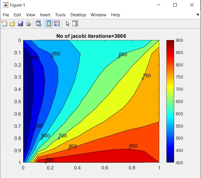
UnSteady state equation using implicit scheme using jacobi iteration method:
clear all
close all
clc
%Solving the steady state 2D heat conduction (Jacobi method)
%Input parameters
nx=10;
ny=10;
nt=1400;
x=linspace(0,1,nx);
y=linspace(0,1,ny);
dx=x(2)-x(1);
dy=dx;
dt=1e-3;
error=9e9;
tol=1e-4;

%defining boundary conditions
left_boundary=400;
right_boundary=800;
top_boundary=600;
bottom_boundary=900;

T=300*ones(nx,ny);
%applying the boundary conditions
T(2:ny-1,1)=left_boundary;
T(1,2:nx-1)=top_boundary;
T(ny,2:nx-1)=bottom_boundary;
T(2:ny-1,nx)=right_boundary;
%calculating average values at the corners
T(1,1)=(left_boundary+top_boundary)/2;
T(nx,ny)=(right_boundary+bottom_boundary)/2;
T(1,ny)=(top_boundary+right_boundary)/2;
T(nx,1)=(left_boundary+top_boundary)/2;
%Assigning original values to T
T_initial=T;
T_old=T;
k1=1.4*(dt/dx^2);
k2=1.4*(dt/dy^2);
jacobi_iteration=1;
for t=1:nt
    error=9e9;
    while(error>tol)
    for i=2:nx-1
        for j=2:ny-1
            term1=1/(1+(2*k1)+(2*k2));
            term2=k1*term1;
            term3=k2*term1;
            H=T_old(i-1,j)+T_old(i+1,j);
            V=T_old(i,j-1)+T_old(i,j+1);
            T(i,j)=(term1*T_initial(i,j))+(term2*H)+(term3*V);
        end
    end
    error=max(max(abs(T_old-T)));
    T_old=T;
    jacobi_iteration=jacobi_iteration+1;
    end
    T_initial=T;

    figure(1)
contourf(x,y,T)
clabel(contourf(x,y,T))
colorbar
colormap
colormap(jet)
set(gca,'ydir','reverse')
title(sprintf('No of jacobi iterations=%d',jacobi_iteration));
xlabel('X-axis')
ylabel('Y-axis')
end
Unsteady state equation using implicit scheme using jacobi iteration method:
clear all
close all
clc
%Solving the steady state 2D heat conduction (gcs)
%Input parameters
nx=10;
ny=10;
nt=1400;
x=linspace(0,1,nx);
y=linspace(0,1,ny);
dx=x(2)-x(1);
dy=dx;
dt=1e-3;
error=9e9;
tol=1e-4;

%defining boundary conditions
left_boundary=400;
right_boundary=800;
top_boundary=600;
bottom_boundary=900;

T=300*ones(nx,ny);
%applying the boundary conditions
T(2:ny-1,1)=left_boundary;
T(1,2:nx-1)=top_boundary;
T(ny,2:nx-1)=bottom_boundary;
T(2:ny-1,nx)=right_boundary;
%calculating average values at the corners
T(1,1)=(left_boundary+top_boundary)/2;
T(nx,ny)=(right_boundary+bottom_boundary)/2;
T(1,ny)=(top_boundary+right_boundary)/2;
T(nx,1)=(left_boundary+top_boundary)/2;
%Assigning original values to T
T_initial=T;
T_old=T;
k1=1.4*(dt/dx^2);
k2=1.4*(dt/dy^2);
Gauss_siedel_iteration=1;
for t=1:nt
    error=9e9;
    while(error>tol)
    for i=2:nx-1
        for j=2:ny-1
            term1=1/(1+(2*k1)+(2*k2));
            term2=k1*term1;
            term3=k2*term1;
            H=T(i-1,j)+T_old(i+1,j);
            V=T(i,j-1)+T_old(i,j+1);
            T(i,j)=(term1*T_initial(i,j))+(term2*H)+(term3*V);
        end
    end
    error=max(max(abs(T_old-T)));
    T_old=T;
    Gauss_siedel_iteration=Gauss_siedel_iteration+1;
    end
    T_initial=T;

    figure(1)
contourf(x,y,T)
clabel(contourf(x,y,T))
colorbar
colormap(jet)
set(gca,'ydir','reverse')
title(sprintf('No of gauss siedel iterations=%d',Gauss_siedel_iteration));
xlabel('X-axis')
ylabel('Y-axis')
end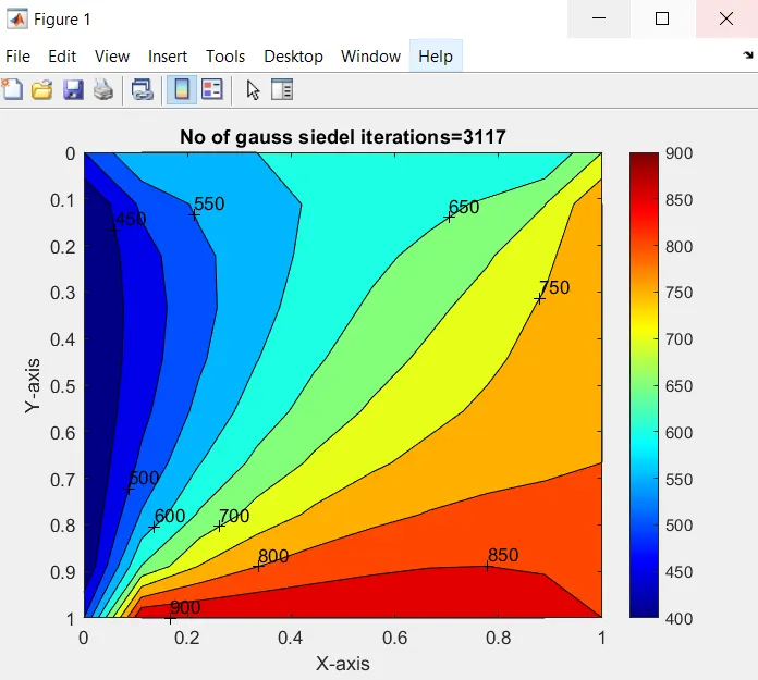
Steady state equation using implicit scheme using Successive over relaxation iteration method:
clear all
close all
clc
%Solving the steady state 2D heat conduction (sor)
%Input parameters
nx=10;
ny=10;
nt=1400;
x=linspace(0,1,nx);
y=linspace(0,1,ny);
dx=x(2)-x(1);
dy=dx;
dt=1e-3;
error=9e9;
tol=1e-4;
omega=1.1;
%defining boundary conditions
left_boundary=400;
right_boundary=800;
top_boundary=600;
bottom_boundary=900;

T=300*ones(nx,ny);
%applying the boundary conditions
T(2:ny-1,1)=left_boundary;
T(1,2:nx-1)=top_boundary;
T(ny,2:nx-1)=bottom_boundary;
T(2:ny-1,nx)=right_boundary;
%calculating average values at the corners
T(1,1)=(left_boundary+top_boundary)/2;
T(nx,ny)=(right_boundary+bottom_boundary)/2;
T(1,ny)=(top_boundary+right_boundary)/2;
T(nx,1)=(left_boundary+top_boundary)/2;
%Assigning original values to T
T_initial=T;
T_old=T;
k1=1.4*(dt/dx^2);
k2=1.4*(dt/dy^2);
Successive_over_relaxation_iteration=1;
for t=1:nt
    error=9e9;
    while(error>tol)
    for i=2:nx-1
        for j=2:ny-1
            term1=1/(1+(2*k1)+(2*k2));
            term2=k1*term1;
            term3=k2*term1;
            H=T(i-1,j)+T_old(i+1,j);
            V=T(i,j-1)+T_old(i,j+1);
            T(i,j)=(omega*((term1*T_initial(i,j))+(term2*H)+(term3*V)))+(1-omega)*(T_old(i,j));
        end
    end
    error=max(max(abs(T_old-T)));
    T_old=T;
   Successive_over_relaxation_iteration=Successive_over_relaxation_iteration+1;
    end
    T_initial=T;

    figure(1)
contourf(x,y,T)
clabel(contourf(x,y,T))
colorbar
colormap(jet)
set(gca,'ydir','reverse')
title(sprintf('No of successive over relaxation iterations=%d',Successive_over_relaxation_iteration));
xlabel('X-axis')
ylabel('Y-axis')
end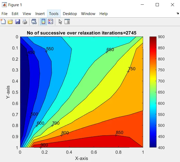
Detailed explanation of the code for unsteady state implicit scheme:
1.The initial conditions and the grid size and the square area is created .
2. The boundary conditions are of the temperature are specified respectively.
3.The corner values of the matrix are calculated accordingly to boundary conditions specified.
4.T_old and T_initial are assigned with the values of T initiallly and time loop is created for x derivative and y derivative,the time loop is also created as the equation varies with time ,the omega value is multiplied for the SOr method alone.
5. The governing equation is written and the error value is calculated and the T_old value is updated for the next iteration,and continues till the error value is less than tolerance value and the T_initial value is updated and end statement for the while loop is closed after plotting the results.
6.Plotting the result in colormap.
Solving unsteady equation using explicit scheme:
delT`/`delt`=`alpha`*(`del^2T`/`delx^2`)+(`del^2T`/`dely^2`)
discretizing the equation we get
(`T_p^(n+1)`-`T_p`)/dt=`alpha*(`(`T_L`-`2T_p`+`T_R`)/`delx^2`) +((`T_T-2T_p+T_B`)/`dely^2`)
If we further simplify
`T_p^(n+1)`=(1/(1+k1+k2))*(`T_p^n`+k1`(T_L+T_R)^(n)`+k2`(T_T+T_B)^(n)`)
where k1=`alpha`*(dt/dx^2), k2=`alpha`*(dt/dy^2)
clear all
close all
clc
%Solving the steady state 2D heat conduction (sor)
%Input parameters
nx=10;
ny=10;
nt=1400;
x=linspace(0,1,nx);
y=linspace(0,1,ny);
dx=x(2)-x(1);
dy=dx;
dt=1e-3;
error=9e9;
tol=1e-4;
omega=1.1;
%defining boundary conditions
left_boundary=400;
right_boundary=800;
top_boundary=600;
bottom_boundary=900;

T=300*ones(nx,ny);
%applying the boundary conditions
T(2:ny-1,1)=left_boundary;
T(1,2:nx-1)=top_boundary;
T(ny,2:nx-1)=bottom_boundary;
T(2:ny-1,nx)=right_boundary;
%calculating average values at the corners
T(1,1)=(left_boundary+top_boundary)/2;
T(nx,ny)=(right_boundary+bottom_boundary)/2;
T(1,ny)=(top_boundary+right_boundary)/2;
T(nx,1)=(left_boundary+top_boundary)/2;
%Assigning original values to T
T_initial=T;
T_old=T;
k1=1.4*(dt/dx^2);
k2=1.4*(dt/dy^2);
explicit=1;
for t=1:nt
    error=9e9;
    while(error>tol)
    for i=2:nx-1
        for j=2:ny-1
            term1=T_old(i,j);
            term2=k1*(T_old(i-1,j)-2*T_old(i,j)+T_old(i+1,j));
            term3=k2*(T_old(i,j-1)-2*T_old(i,j)+T_old(i,j+1));
            T(i,j)=term1+term2+term3;
        end
    end
    error=max(max(abs(T_old-T)));
    T_old=T;
  explicit=explicit+1;

    end
end


figure(1)
contourf(x,y,T)
clabel(contourf(x,y,T))
colorbar
colormap(jet)
set(gca,'ydir','reverse')
title(sprintf('No of explicit iterations=%d',explicit));
xlabel('X-axis')
ylabel('Y-axis')
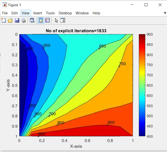
Results and conclusion:
| Types of scheme and analysis | various methods | No .of iterations |
| implicit steady state | jacobi | 208 |
| implicit steady state | Gauss seidel | 112 |
| implicit steady state | SOR | 60 |
| implicit unsteady | jacobi | 3666 |
| implicit unsteady | Gauss seidel | 3117 |
| implicit unsteady | Sor | 2745 |
| explicit scheme | 1833 |
from the above obtained results of various methods and comparing the no. of iterations
Jacobi>Gauss seidel>SOR according to the no.of iterations compared to all methods and schemes
While comparing steay state and unsteady state ,it is proven that steady state is more efficient as it takes less no.of iterations.
In transient equations with explicit scheme method yields the result quickly compared to implicit method ,but is recommended in situation when CFL is under 0.25