Week 3 - Adiabatic Flame Temperature calculation
Aim :
To find the Adiabatic flame temperature on equivalence ratio with different Hydrocarbons and for different alkanes with heat loss (In constant pressure chamber)and without heat loss.
Adiabatic flame temperature variation with respect to Alkane,Alkene,Alkyne.
Adiabatic flame temperature variation with respect to number of Carbon atom chains.
Adiabatic flame Temperature:
The adiabatic flame temperature is defined as the temperature attained when all of the chemical reaction heat released heats combustion products.
If no heat is lost in this process, the temperature of the combustion products is known as the "Adiabatic Flame Temperature."=
Equivalence ratio:
The measure of how a mixture is derivating from an ideal stoichiometric reaction.
If Equivalence ratio =1 it is stoichiometric mixture.
If Equivalence ratio >1 it is rich mixture.
If Equivalence ratio <1 it is lean mixture.
General equation for Hydrocarbon reaction:
`C_xH_y + [x+(y/4)](O_2 + 3.762N_2 => xCo_2 + (y/2)H_2O + 3.76[x + (y/4)]N_2`
Chemical reaction for combustion of methane:
Stoichiometric combustion:
`CH_4 + 2(O_2 + 3.762N_2) => CO_2 +2H_2O +7.52N_2`
Lean combustion:
`CH_4 +(2/phi)(O_2 +3.76N_2) => CO_2 + 2H_2o + (2/phi-2)O_2 +(7.52/phi)N_2)`
Rich combustion:
`CH_4 +(2/phi)(O_2 +3.76N_2) => (4/phi-3)CO_2 + 2H_2o + (4-4/phi)CO +(7.52/phi)N_2)`
Case 1: EFFECT OF EQUIVALENCE RATIO ON AFT FOR COMBUSTION OF METHANE UNDER CONSTANT VOLUME COMBUSTION PROCESS
For a constant volume process, the internal energy is equated for reactants and products to get AFT.
`U_r - U_p =0`
So using newton's raphson method the final temperature is obtained.
`(H_(pr oducts)- n_(pr oducts)*R*T) - (H_(reactants)-n_(reactants)*R*T_(std))`
import matplotlib.pyplot as plt
import math
import numpy as np

def h(T,co_effs):
	R = 8.314 #J/mol-k
	a1 = co_effs[0]
	a2 = co_effs[1]
	a3 = co_effs[2]
	a4 = co_effs[3]
	a5 = co_effs[4]
	a6 = co_effs[5]

	return (a1 + a2*T/2 + a3*pow(T,2)/3 + a4*pow(T,3)/4 + a5*pow(T,4)/5 + a6/T)*R*T
	#low temperature coefficient
ch4_coeffs_l = [5.14987613E+00,-1.36709788E-02,4.91800599E-05,-4.84743026E-08,1.66693956E-11,-1.02466476E+04,-4.64130376E+00]
o2_coeffs_l = [3.78245636E+00,-2.99673416E-03,9.84730201E-06,-9.68129509E-09,3.24372837E-12,-1.06394356E+03,3.65767573E+00]
n2_coeffs_l = [0.03298677E+02,0.14082404E-02,-0.03963222E-04,0.05641515E-07,-0.02444854E-10,-0.10208999E+04,0.03950372E+02]
	#High temperature coefficients
o2_coeffs_h = [3.28253784E+00,1.48308754E-03,-7.57966669E-07,2.09470555E-10,-2.16717794E-14,-1.08845772E+03,5.45323129E+00]
n2_coeffs_h = [0.02926640E+02,0.14879768E-02,-0.05684760E-05,0.10097038E-09,-0.06753351E-13,-0.09227977E+04,0.05980528E+02]
co2_coeffs_h = [3.85746029E+00,4.41437026E-03,-2.21481404E-06,5.23490188E-10,-4.72084164E-14,-4.87591660E+04,2.27163806E+00]
h2o_coeffs_h = [3.03399249E+00,2.17691804E-03,-1.64072518E-07,-9.70419870E-11,1.68200992E-14,-3.00042971E+04,4.96677010E+00]
co_coeffs_h = [2.71518561E+00,2.06252743E-03,-9.98825771E-07,2.30053008E-10,-2.03647716E-14,-1.41518724E+04,7.81868772E+00]

def f(T):
	h_co2_p = h(T,co2_coeffs_h)
	h_n2_p = h(T,n2_coeffs_h)
	h_h2o_p = h(T,h2o_coeffs_h)
	h_o2_p = h(T,o2_coeffs_h)
	h_co_p = h(T,co_coeffs_h)

	R = 8.314

	#lean mixture
	if phi < 1:
		H_products = h_co2_p +2*h_h2o_p + (7.52/phi)*h_n2_p + ((2/phi)-2)*h_o2_p

		n_products = 1 + (7.52/phi) + 2 + ((2/phi)-2)

	if phi == 1:
		H_products = h_co2_p + 2*h_h2o_p +7.52*h_n2_p
		n_products = 1 +7.52 +2

	#rich mixture
	if phi > 1:
		H_products = ((4/phi)-3)*h_co2_p + 2*h_h2o_p + (7.52/phi)*h_n2_p +(4-(4/phi))*h_co_p
		n_products = ((4/phi)-3) + (7.52/phi) + 2 + (4-(4/phi))

	Tstd = 298.15
	h_ch4_r = h(Tstd,ch4_coeffs_l)
	h_o2_r = h(Tstd,o2_coeffs_l)
	h_n2_r = h(Tstd,n2_coeffs_l)

	H_reactants = h_ch4_r + (2/phi)*(h_o2_r + (3.76*h_n2_r))
	n_reactants = 1 + (2/phi) + 3.76*(2/phi)

	return (H_products - n_products*R*T) - (H_reactants - n_reactants*R*Tstd)

def fprime(T):
	return (f(T+1e-6) - f(T))/1e-6

#Newton raphson method
T_guess = 1500
tol = 1e-03
alpha = 0.2
X = np.arange(0.1,2,0.05)
T_ad = []

for phi in X:
	while(abs(f(T_guess))>tol):
		T_guess = T_guess - alpha*((f(T_guess)/fprime(T_guess)))

	T_ad.append(T_guess)


import cantera as ct
T_adc = []
for phi in np.arange(0.1,2,0.05):  ####np.arange not np.arra
	gas = ct.Solution('gri30.xml')
	gas.TPX =298.15,101325,{'CH4':1,'O2':2/phi,'N2':7.52/phi}
	gas.equilibrate('UV','auto')
	T_adc.append(gas.T)

#plotting
plt.plot(X,T_ad,color='red',label="using newton raphson")
plt.plot(X,T_adc,color='blue',label="using cantera")
plt.xlabel('Equivalence ratio')
plt.ylabel('Adiabatic Flame Temperature')
plt.title('Effect of Equivalence ratio on Aft on Methane')
plt.legend()
plt.grid('on')
plt.show()
In this case we take methane combustion as an example.At first we solved for various species of fuel reactions.Then phi is defined ,after which we input all the reactions and lean mixture chemical reactions .Then we define the derivative function to solve equation by Newton raphson method to obtain Adiabatic flame temperature for methane gas.Then the problem is solved in cantera to see results compared with python code.
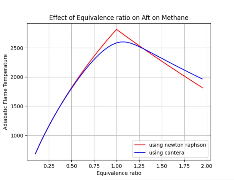
Here we can see that python code does not include all species involved in combustion process but cantera takes all into account.So cantera result is said to be more accurate.
Case 2: Flame temperature variation with heat loss
Here we consider a constant pressure reactor with heat loss. The reactor is initially set at STP conditions.Here the code is similar to the previous code with a heat loss parameter H_loss is added to the function to compute the reactions.
import matplotlib.pyplot as plt
import math
import numpy as np

x=1
y=4
R=8.314
Qs=802000  #As product are at gas phase Qs =LHV'mf = 50*e+6*16.04*e-3

H_loss = np.linspace(0,1,20)
H_product =[]
H_reactanats =[]
def h(T, co_effs):

	R=8.314
	a1= co_effs[0]
	a2= co_effs[1]
	a3= co_effs[2]
	a4= co_effs[3]
	a5= co_effs[4]
	a6= co_effs[5]

	return (a1 + a2*T/2+a3*pow(T,2)/3+a4*pow(T,3)/4+a5*pow(T,4)/5 +a6/T)*R*T

ch4_coeffs_l = [5.14987613E+00, -1.36709788E-02, 4.91800599E-05, -4.84743026E-08,1.66693956E-11, -1.02466476E+04, -4.64130376E+00]
o2_coeffs_l = [3.78245636E+00 ,-2.99673416E-03, 9.84730201E-06,-9.68129509E-09, 3.24372837E-12,-1.06394356E+03 ,3.65767573E+00]
n2_coeffs_l= [ 0.03298677E+02, 0.14082404E-02,-0.03963222E-04, 0.05641515E-07,-0.02444854E-10,-0.10208999E+04 ,0.03950372E+02]
n2_coeffs_h=[0.02926640E+02 ,0.14879768E-02,-0.05684760E-05 ,0.10097038E-09,-0.06753351E-13,-0.09227977E+04, 0.05980528E+02]
co2_coeffs_h=[3.85746029E+00,4.41437026E-03,-2.21481404E-06, 5.23490188E-10,-4.72084164E-14 ,-4.87591660E+04 ,2.27163806E+0]
o2_coeffs_h= [3.28253784E+00, 1.48308754E-03,-7.57966669E-07, 2.09470555E-10,-2.16717794E-14,-1.08845772E+03,5.45323129E+00]
co_coeffs_h=[2.71518561E+00 ,2.06252743E-03,-9.98825771E-07,2.30053008E-10,-2.03647716E-14,-1.41518724E+04, 7.81868772E+00]
h20_coeffs_h=[3.03399249E+00 ,2.17691804E-03,-1.64072518E-07,-9.70419870E-11 ,1.68200992E-14,-3.00042971E+04 ,4.96677010E+00]
def f(T,H_loss):

	h_co2_p=h(T,co2_coeffs_h)
	h_h20_p=h(T,h20_coeffs_h)
	h_n2_p=h(T,n2_coeffs_h)
	H_product = h_co2_p +2*h_h20_p +7.52*h_n2_p
	Tstd = 298.15
	h_ch4_r= h(Tstd,ch4_coeffs_l)
	h_o2_r=h(Tstd,o2_coeffs_l)
	h_n2_r=h(Tstd,n2_coeffs_l)
	H_reactants=h_ch4_r +2*h_o2_r + 7.52*h_n2_r

	return H_product - H_reactants + (H_loss*Qs)

	#Newton Raphson method
def fprime(T,H_loss):
	return(f(T+1e-6,H_loss)-f(T,H_loss))/1e-06

tol = 1e-3
alpha = 0.9
Temp=[]

for i in H_loss:
	T_guess =1500
	R=8.314

	while(abs(f(T_guess,i))>tol):
		T_guess =T_guess - alpha*((f(T_guess,i)/fprime(T_guess,i)))


	Temp. append(T_guess)

print(Temp)
T_loss = (Temp[10])
print(T_loss)

plt.figure(1)
plt.plot(H_loss,Temp,color = 'yellow')
plt.xlabel('H loss coefficient')
plt.ylabel('Adiabatic flame Temperature')
plt.title('Effect of AFT on Equivalence Ratio with heat loss')
plt.grid()
plt.show()
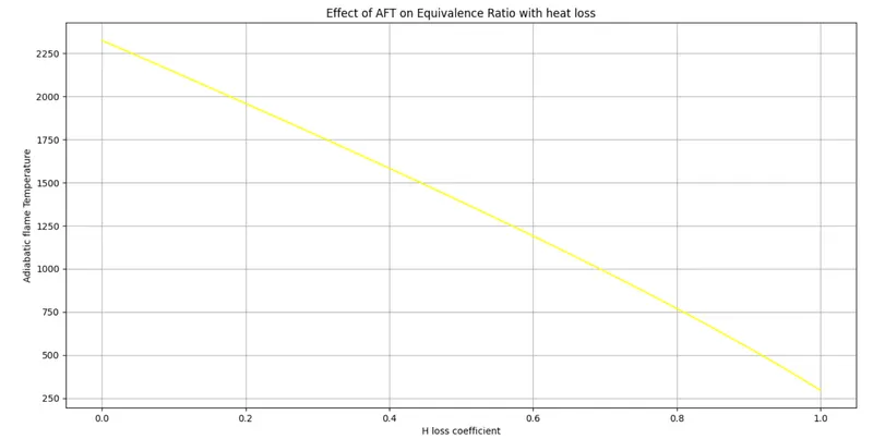
As the heat loss coefficient increases from 0 to 1 we can see that there is minimum heat loss due to heat loss coefficient parameter.
Case 3: Adiabatic flame temperature variation with respect to Alkane, Alkene, Alkyne :
Here we wrote a code in cantera to compute adiabatic flame temperature for different forms of hydrocarbon.At first we used the gas solving library and we defined the different forms of hydrocarbons.The gas.TPX command is used to define STP conditions at the beginning of the combustion process.In this case we are computing the enthalpies of the different forms of hydrocarbon and comparing them.
import matplotlib.pyplot as plt
import numpy as np
import cantera as ct

gas = ct.Solution('gri30.xml')

gas.TPX = 298.15,101325,{'C2H2':1,'O2':3.5,'N2':9.4}
gas.equilibrate('HP','auto')
T_c2h2 =gas.T

gas.TPX = 298.15,101325,{'C2H4':1,'O2':3.5,'N2':11.28}
gas.equilibrate('HP','auto')
T_c2h4 =gas.T

gas.TPX = 298.15,101325,{'C2H6':1,'O2':3.5,'N2':13.16}
gas.equilibrate('HP','auto')
T_c2h6 =gas.T

temp = (T_c2h2,T_c2h4,T_c2h6)
temp = np.array(temp)
print(temp)

plt.figure()
plt.bar(['C2H2','C2H4','C2H6'],temp,color = 'red')
plt.xlabel('Fuel species')
plt.ylabel('Adiabatic Flame Temperature')
plt.title('AFT vs Fuel type')
plt.show() 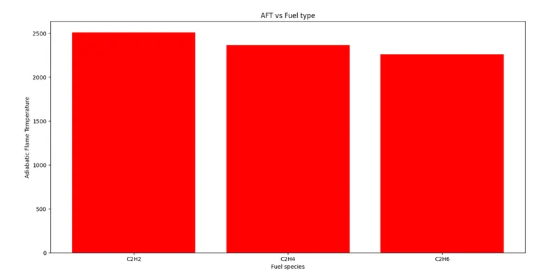
Case 4:Adiabatic flame temperature variation with respect to number of Carbon atom chains :
import matplotlib.pyplot as plt
import math
import numpy as np

def h(T,co_effs):

       R=8.314
       a1= co_effs[0]
       a2= co_effs[1]
       a3= co_effs[2]
       a4= co_effs[3]
       a5= co_effs[4]
       a6= co_effs[5]

       return (a1 + a2*T/2+a3*pow(T,2)/3+ a4*pow(T,3)/4+ a5*pow(T,4)/5 +a6/T)*R*T

ch4_coeffs_l =[5.14987613E+00,-1.36709788E-02,4.91800599E-05,-4.84743026E-08, 1.66693956E-11,-1.02466476E+04,-4.64130376E+00]
c2h6_coeffs_l = [4.29142492E+00,-5.50154270E-03,5.99438288E-05,-7.08466285E-08, 2.68685771E-11,-1.15222055E+04, 2.66682316E+00]
c3h8_coeffs_l = [0.93355381E+00, 0.26424579E-01, 0.61059727E-05,-0.21977499E-07, 0.95149253E-11,-0.13958520E+05, 0.19201691E+02]
o2_coeffs_l = [3.78245636E+00,-2.99673416E-03, 9.84730201E-06,-9.68129509E-09, 3.24372837E-12,-1.06394356E+03,3.65767573E+00]
n2_coeffs_l = [0.03298677E+02 ,0.14082404E-02,-0.03963222E-04,0.05641515E-07,-0.02444854E-10,-0.10208999E+04,0.03950372E+02]
n2_coeffs_h = [0.02926640E+02 ,0.14879768E-02,-0.05684760E-05, 0.10097038E-09,-0.06753351E-13,-0.09227977E+04, 0.05980528E+02, 0.03298677E+02]
co2_coeffs_h = [3.85746029E+00, 4.41437026E-03,-2.21481404E-06, 5.23490188E-10,-4.72084164E-14,-4.87591660E+04, 2.27163806E+00, 2.35677352E+00]
h2o_coeffs_h = [3.03399249E+00,2.17691804E-03,-1.64072518E-07,-9.70419870E-11 ,1.68200992E-14,-3.00042971E+04,4.96677010E+00]
Tstd = 298.15
H1 = h(Tstd,ch4_coeffs_l)
H2 = h(Tstd,c2h6_coeffs_l)
H3 = h(Tstd,c3h8_coeffs_l)
H =[H1,H2,H3]
H = np.array(H)
def f(T,H):

     h_co2_p = h(T,co2_coeffs_h)
     h_h2o_p = h(T,h2o_coeffs_h)
     h_n2_p = h(T,n2_coeffs_h)
     h_o2_r = h(T,o2_coeffs_l)
     h_n2_r = h(T,n2_coeffs_l)

     if H == H1:
            x = 15
            y = 4
            a =x +(y/4)
            H_product = x*h_co2_p + (y/2)*h_h2o_p +(3.76*a)*h_n2_p
            H_reactants = H1 + a*h_o2_r + (3.76*a)*h_n2_r
     elif H == H2:
            x = 2
            y = 6
            a =x +(y/4)
            H_product = x*h_co2_p + (y/2)*h_h2o_p +(3.76*a)*h_n2_p
            H_reactants = H2 + a*h_o2_r + (3.76*a)*h_n2_r
     elif H == H3:
            x = 3
            y = 8
            a =x +(y/4)
            H_product = x*h_co2_p + (y/2)*h_h2o_p +(3.76*a)*h_n2_p
            H_reactants = H3 + a*h_o2_r + (3.76*a)*h_n2_r

     return H_product - H_reactants

def fprime(T,H):
       return(f(T+1e-6,H) - f(T,H))/1e-6

T_guess = 1500
tol = 1e-3
ct = 0
alpha =0.9
temp = []

for i in H:
       T_guess = 1500
       R=8.314

       while(abs(f(T_guess,i))>tol):
              T_guess =T_guess - alpha*((f(T_guess,i)/fprime(T_guess,i)))

       temp. append(T_guess)
       print(T_guess)
plt.figure()
plt.bar(['CH4','C2H6','C3H8'],temp,color = 'blue')
plt.xlabel('Fuel Species')
plt.ylabel('Adiabatic flame Temperature')
plt.title('Effect of number of Carbon atoms')
plt.show()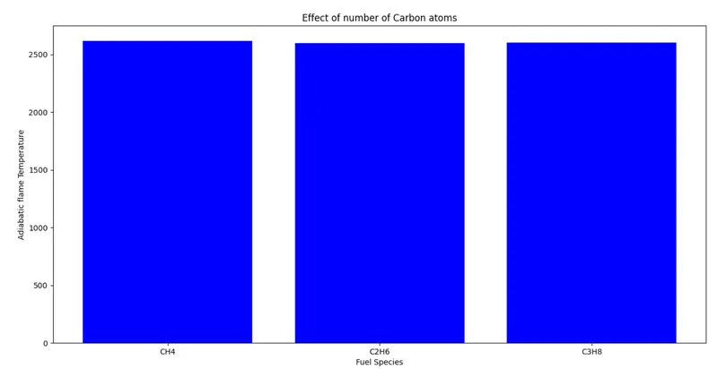
Conclusion:
1. The effect of equivalence ratio with AFT
2. Effects like Heat loss ,Aft compared with different fuel species and number of carbon atoms are also observed.
3. Comparison of Python and cantera solvers were made ,cantera predicts results with accuracy then python.