Week 3.5 - Deriving 4th order approximation of a 2nd order derivative using Taylor Table method

Objective

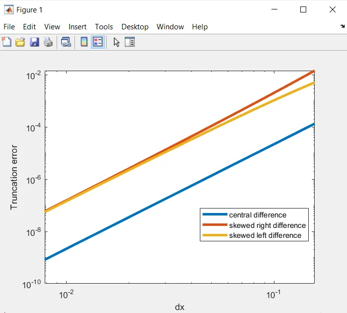
To find the 4th order approximations of the second-order derivative. Central difference Skewed right-sided difference Skewed left-sided difference and compare their truncation error.

Taylor table for central difference scheme:

The 4th order central difference of the second order derivative ,by using Taylor's method

`del^2f`/`delx^2`=af(i-2)+bf(i-1)+cf(i)+df(i+1)+ef(i+2)

for central differencing , n=p+q-1, here n- no of nodes, p-order of derivative, q-order of approximation

Taylor table for central difference

	f(x)	dx f'(x)	`dx^2f''(x)`	`dx^3f'''(x)`	dx^4f''''(x)	dx^5f'''''(x)
af(i-2)	a	-2a	4a/2	-8a/6	16a/24	-32a/120
bf(i-1)	b	-b	b/2	-b/6	b/24	-b/120
cf(i)	c	0	0	0	0	0
df(i+1)	d	d	d/2	d/6	d/24	d/120
ef(i+2)	e	2e	4e/2	8e/6	16e/24	32e/120
`sum`	0	0	1	0	0

Converting table in to matrix form AX=B, and extracting equations

a+b+c+d+e=0

-2a+-b+d+2e=0

4a/2+b/2+d/2+4e/2=1

-8a/6-b/6+d/6+8e/6=0

16a/24+b/24+d/24+16e/24=0

by solving the above equations we get

a=-0.0833,b=1.3333,c=-2.5,d=1.3333,e=-0.08333

Skewed right sided difference

the 4th order skewed right sided difference , for skewed differencing n=p+q

`del^2f`/`delx^2`=af(i)+bf(i+1)+cf(i+2)+df(i+3)+ef(i+4)+gf(i+5)

taylor table for skewed differncing

	f(x)	dx f'(x)	`dx^2f''(x)`	`dx^3f'''(x)`	dx^4f''''(x)	dx^5f'''''(x)
af(i)	a	0	0	0	0	0
bf(i+1)	b	b	b/2	b/6	b/24	b/120
cf(i+2)	c	2c	4c/2	8c/6	16c/24	32c/120
df(i+3)	d	3d	9d/2	27d/6	81d/24	243d/120
ef(i+4)	e	4e	16e/2	64e/6	256e/24	1024e/120
gf(i+5)	g	5g	25g/2	125g/6	625g/24	3125g/120
`sum`	0	0	1	0	0	0

converting to matrix form and and extracting equation

a+b+c+d+e+g=0

b+2c+3d+4e+5g=0

b/2+4c/2+9d/2+16e/2+25g/2=1

b/6+8c/6+27d/6+64e/6+125g/6=0

b/24+16c/24+81d/24+256e/24+625g/24=0

by solving the above equations we get

a=3.75,b=-12.8333,c=17.833,d=-13,e=5.0833,f=-0.8333

Skewed left sided difference

the 4th order skewed right sided difference , for skewed differencing n=p+q

`del^2f`/`delx^2`=af(i-5)+bf(i-4)+cf(i-3)+df(i-2)+ef(i-1)+gf(i)

taylor table for skewed differncing

	f(x)	dx f'(x)	`dx^2f''(x)`	`dx^3f'''(x)`	dx^4f''''(x)	dx^5f'''''(x)
af(i-5)	a	-5a	25a/2	-125a/6	625a/24	-3125a/120
bf(i-4)	b	-4b	16b/2	-64b/6	256b/24	-1024b/120
cf(i-3)	c	-3c	9c/2	-27c/6	81c/24	-243c/120
df(i-2)	d	-2d	4d/2	-8d/6	16d/24	-32d/120
ef(i-1)	e	-e	e/2	-e/6	e/24	-e/120
gf(i)	g	0	0	0	0	0
`sum`	0	0	1	0	0	0

by converting the above table matrix form and extracting equations we get

a+b+c+d+e+g=0

-5a-4b-3c-2d-e=0

25a/2+ 16b/2 +9c/2 +4d/2 +e/2=1

-125a/6 -64b/6 -27c/6- 8d/6 -e/6=0

625a/24 +256b/24 +81c/24 +16d/24 +e/24 =0

-3125a/120 -1024b/120 -243c/120 -32d/120 -e/120 =0

by solving he above equations we get

a=-0.8333,b=5.0833, c=13, d=17.833, e=-12.833, f=3.75

Procedure to follow to achieve the objectives:

1.We assign the values for x and dx

2.We define anonymous function of analytical function and its derivative

3. We derived taylor series for central differencing, skewed right differencing and skewed left differencing for the analytical function and tabulated all the coefficients for different order of derivatives

4.We sum all the tabulated values

4. Converted the tabulated coefficient values to matrix form and using inversion we solve all the equations and found values for the coefficients.

5.loop the order of approximation expression in for loop under range of dx.The absolute error is calculated from the derivative value calculated analyticallly.

6.the error are plotted on graph to do a better comparison

clear all
close all
clc
%inputs
x=pi/3;
dx=linspace(pi/20,pi/400,20);
%finding central differencing
A=[1 1 1 1 1;-2 -1 0 1 2;4/2 1/2 0 1/2 4/2;-8/6 -1/6 0 1/6 8/6;16/24 1/24 0 1/24 16/24];
B=[0;0;1;0;0];
X=inv(A)*B;
%finding right skewed difference
C=[1 1 1 1 1 1;0 1 2 3 4 5;0 1/2 4/2 9/2 16/2 25/2;0 1/6 8/6 27/6 64/6 125/6;0 1/24 16/24 81/24 256/24 625/24;0 1/120 32/120 243/120 1024/120 3125/120];
D=[0;0;1;0;0;0];
Y=inv(C)*D;
%finding left skewed difference
E=[1 1 1 1 1 1;-5 -4 -3 -2 -1 0;25/2 16/2 9/2 4/2 1/2 0;-125/6 -64/6 -27/6 -8/6 -1/6 0;625/24 256/24 81/24 16/24 1/24 0;-3125/120 -1024/120 -243/120 -32/120 -1/120 0];
F=[0;0;1;0;0;0];
Z=inv(E)*F;

for i=1:length(dx)
    central_error(i)=central_differencing(x,dx(i),X);
    right_error(i)=right_skewed_differencing(x,dx(i),Y);
    left_error(i)=left_skewed_differencing(x,dx(i),Z);
end
figure(1)
loglog(dx,central_error,'linewidth',3);
hold on
loglog(dx,right_error,'linewidth',3);
hold on
loglog(dx,left_error,'linewidth',3);
hold off
xlabel('dx')
ylabel('Truncation error')
legend('central difference','skewed right difference','skewed left difference')

%function for central differencing
function error=central_differencing(x,dx,X)
exact_derivative=-2*exp(x)*sin(x);
%writing the central differncing taylor series 
%af(i-2)+bf(i-1)+cf(i)+df(i+1)+ef(i+2)
f1=exp(x-2*dx)*cos(x-2*dx);
f2=exp(x-dx)*cos(x-dx);
f3=exp(x)*cos(x);
f4=exp(x+dx)*cos(x+dx);
f5=exp(x+2*dx)*cos(x+2*dx);

central_difference=((X(1)*f1)+(X(2)*f2)+(X(3)*f3)+(X(4)*f4)+(X(5)*f5))/(dx^2);
error=abs(central_difference-exact_derivative);
end
%function for skewed right differencing
function error=right_skewed_differencing(x,dx,Y)
exact_derivative=-2*exp(x)*sin(x);
%writing the central differncing taylor series 
%af(i)+bf(i+1)+cf(i+2)+df(i+3)+ef(i+4)+gf(i+5)
f1=exp(x)*cos(x);
f2=exp(x+dx)*cos(x+dx);
f3=exp(x+2*dx)*cos(x+2*dx);
f4=exp(x+3*dx)*cos(x+3*dx);
f5=exp(x+4*dx)*cos(x+4*dx);
f6=exp(x+5*dx)*cos(x+5*dx);
right_difference=((Y(1)*f1)+(Y(2)*f2)+(Y(3)*f3)+(Y(4)*f4)+(Y(5)*f5)+(Y(6)*f6))/(dx^2);
error=abs(right_difference-exact_derivative);
end

%function for skewed left differencing
function error=left_skewed_differencing(x,dx,Z)
exact_derivative=-2*exp(x)*sin(x);
%writing the central differncing taylor series 
%af(i-5)+bf(i-4)+cf(i-3)+df(i-2)+ef(i-1)+gf(i)
f1=exp(x-5*dx)*cos(x-5*dx);
f2=exp(x-4*dx)*cos(x-4*dx);
f3=exp(x-3*dx)*cos(x-3*dx);
f4=exp(x-2*dx)*cos(x-2*dx);
f5=exp(x-dx)*cos(x-dx);
f6=exp(x)*cos(x);
left_difference=((Z(1)*f1)+(Z(2)*f2)+(Z(3)*f3)+(Z(4)*f4)+(Z(5)*f5)+(Z(6)*f6))/(dx^2);
error=abs(left_difference-exact_derivative);
end

Results

From the observed result we can see that the skewed right difference and skewed left difference is almost same,the truncation error of the cental difference is less compared to skewed right and left difference,because the central differnce takes values from both sides of the grid points so the numerical approximation is bettre than the other two schemes.