Week 11 - Simulation of Flow through a pipe in OpenFoam
Objective:
To simulate an axi-symmetric flow by applying the wedge boundary condition. The flow is laminar and flows through a constant cross-section pipe at an inlet Reynold's number of 2100.
To write code in Matlab to automate the generation of blockMeshDict file. The code should take inputs like pipe length, diameter, wedge angle, etc and output a fully functional blockMeshDict file.
The final objective is to post process the results of velocity at different length of pipe and shear stress at fully developed portion and compare it with analytical solution.
Assumptions:
- Steady flow ,incompressible and laminar flow.
- Constant fluid properties
- Two dimensional flow.
Laminar flow through pipe:
Flow in pipes is laminar for Re ≲ 2300, and that the flow is fully developed if the pipe is sufficiently long (relative
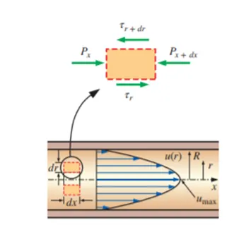
to the entry length) so that the entrance effects are negligible.we consider the steady, laminar, incompressible flow of fluid with constant properties in the fully developed region of a straight circular pipe.
The average velocity
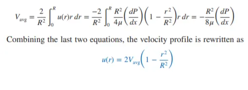
The maximum velocity occurs at the centreline 
Reynolds Number:
The transition from laminar to turbulent flow depends on the geometry, surface roughness, flow velocity, surface temperature, and type of fluid, among other things.The ratio of inertial forces to viscous forces in the fluid (Fig. 8–5). This ratio is called the Reynolds number.The flow in a circular pipe is laminar for Re ≲ 2300, turbulent for Re ≳ 4000,
and transitional in between.

HydroDynamic length:
The region from the pipe inlet to the point at which the velocity boundary layer merges at the centre line is called hydrodynamic entrance region.The region beyond the entrance region in which velocity profile fully developed is called fully developed region.
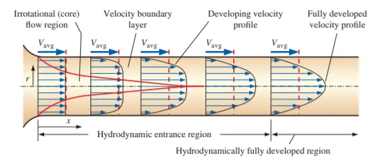
In laminar flow entry length is given as 0.06.Re.D.
Hagen poiseuille flow:
For a specified flow rate, the pressure drops and thus the required pumping power is proportional to the length of the pipe and the viscosity of the fluid, but it is inverselyproportional to the fourth power of the radius (or diameter) of the pipe.
Pressure Drop:

Working fluid (Water) Kinematic viscosity: 1e-06m^2/s
Dynamic viscosity: mu = 0.89*10^-3 Pa.s
Density of water = 1000 Kg/m^3
Reynolds Number =2100
average velocity = 0.09345m/s
V_max= 2*v_avg= 0.1869 m/s
Matlabcode for blkMeshDict:
close all
clear all
clc

%input conditions
Re=2100; %given
D=0.02; %assumption in meters
R=D/2;
rho=1000; %density for water
entry_length= 0.06*Re*D; %hydrodynamic entry length
mu=0.00089; % viscosity in Pa.s
nu=mu/rho; %kinematic viscosity
theta=4;%angle less than 5 degrees

%boundary conditions
v_avg=(Re*nu)/D;
v_max=2*v_avg;
L=entry_length+0.3; %total length of pipe
delta_p=(8*mu*L*v_avg)/R^2; %pressure drop

%vertices co-ordinates
v0=[0 0 0];
v1=[0 R*cosd(theta/2) R*sind(theta/2)];
v2=[0 R*cosd(theta/2) -R*sind(theta/2)];
v3=[L 0 0];
v4=[L R*cosd(theta/2) R*sind(theta/2)];
v5=[L R*cosd(theta/2) -R*sind(theta/2)];


h1='/*--------------------------------*- C++ -*----------------------------------*\';
h2='  =========                 |                                                  ';
h3='  \\      /  F ield         | OpenFOAM: The Open Source CFD Toolbox            ';
h4='   \\    /   O peration     | Website:  https://openfoam.org                   ';
h5='    \\  /    A nd           | Version:  8                                      ';
h6='     \\/     M anipulation  |                                                  ';
h7='\*---------------------------------------------------------------------------*/';

f1=fopen('blockMeshDict.txt','w')

fprintf(f1,'%s \n',h1);
fprintf(f1,'%s \n',h2);
fprintf(f1,'%s \n',h3);
fprintf(f1,'%s \n',h4);
fprintf(f1,'%s \n',h5);
fprintf(f1,'%s \n',h6);
fprintf(f1,'%s \n',h7);

fprintf(f1, 'FoamFile \n {\n');
fprintf(f1,'%12s \t 2.0;\n','version');
fprintf(f1,'%12s \t ascii;\n','format');
fprintf(f1,'%12s \t dictionary;\n','class');
fprintf(f1,'%12s \t blockMeshDict;\n','object');
fprintf(f1,'}\n');
fprintf(f1,'// * * * * * * * * * * * * * * * * * * * * * * * * * * * * * * * * *// \n');
fprintf(f1,'convertToMeters 1;\n\n');
fprintf(f1,'vertices\n(\n');
fprintf(f1,'\t(%d %d %d)\n',v0);
fprintf(f1,'\t(%d %d %d)\n',v1);
fprintf(f1,'\t(%d %d %d)\n',v2);
fprintf(f1,'\t(%d %d %d)\n',v3);
fprintf(f1,'\t(%d %d %d)\n',v4);
fprintf(f1,'\t(%d %d %d)\n',v5);
fprintf(f1,');\n\n');

fprintf(f1,'blocks\n(\n');
fprintf(f1,'\t hex(0 3 5 2 0 3 4 1) (%d %d %d)',200,20,1);
fprintf(f1,' simpleGrading (1 0.1 1)\n);\n \n');

fprintf(f1,'edges\n(\n');
fprintf(f1,'\t arc %d %d (%d %d %d)\n',1,2,0,R,0);
fprintf(f1,'\t arc %d %d (%d %d %d)\n',4,5,L,R,0);
fprintf(f1,');\n\n');

fprintf(f1,'boundary\n');
fprintf(f1,'(\n');
fprintf(f1,'\t inlet\n');
fprintf(f1,'\t {\n');
fprintf(f1,'\t\t type patch;\n');
fprintf(f1,'\t\t faces\n');
fprintf(f1,'\t\t (\n');
fprintf(f1,'\t\t\t (0 1 2 0)\n');
fprintf(f1,'\t\t );\n');
fprintf(f1,'\t }\n');

fprintf(f1,'\t outlet\n');
fprintf(f1,'\t {\n');
fprintf(f1,'\t\t type patch;\n');
fprintf(f1,'\t\t faces\n');
fprintf(f1,'\t\t (\n');
fprintf(f1,'\t\t\t (3 5 4 3)\n');
fprintf(f1,'\t\t );\n');
fprintf(f1,'\t }\n');

fprintf(f1,'\t top\n');
fprintf(f1,'\t {\n');
fprintf(f1,'\t\t type wall;\n');
fprintf(f1,'\t\t faces\n');
fprintf(f1,'\t\t (\n');
fprintf(f1,'\t\t\t (1 4 5 2)\n');
fprintf(f1,'\t\t );\n');
fprintf(f1,'\t }\n');

fprintf(f1,'\t front\n');
fprintf(f1,'\t {\n');
fprintf(f1,'\t\t type wedge;\n');
fprintf(f1,'\t\t faces\n');
fprintf(f1,'\t\t (\n');
fprintf(f1,'\t\t\t (0 3 4 1)\n');
fprintf(f1,'\t\t );\n');
fprintf(f1,'\t }\n');

fprintf(f1,'\t back\n');
fprintf(f1,'\t {\n');
fprintf(f1,'\t\t type wedge;\n');
fprintf(f1,'\t\t faces\n');
fprintf(f1,'\t\t (\n');
fprintf(f1,'\t\t\t (0 2 5 3)\n');
fprintf(f1,'\t\t );\n');
fprintf(f1,'\t }\n');

fprintf(f1,'\t axis\n');
fprintf(f1,'\t {\n');
fprintf(f1,'\t\t type empty;\n');
fprintf(f1,'\t\t faces\n');
fprintf(f1,'\t\t (\n');
fprintf(f1,'\t\t\t (0 3 3 0)\n');
fprintf(f1,'\t\t );\n');
fprintf(f1,'\t }\n');

fprintf(f1,'mergePatchPairs\n');
fprintf(f1,'(\n');
fprintf(f1,');\n');

fprintf(f1,'// * * * * * * * * * * * * * * * * * * * * * * * * * * * * * * * * *// \n');
fclose(f1)
/*--------------------------------*- C++ -*----------------------------------*\
========= |
\\ / F ield | OpenFOAM: The Open Source CFD Toolbox
\\ / O peration | Website: https://openfoam.org
\\ / A nd | Version: 8
\\/ M anipulation |
\*---------------------------------------------------------------------------*/
FoamFile
{
version 2.0;
format ascii;
class dictionary;
location "system";
object controlDict;
}
// * * * * * * * * * * * * * * * * * * * * * * * * * * * * * * * * * * * * * //
application icoFoam;
startFrom startTime;
startTime 0;
stopAt endTime;
endTime 5;
deltaT 0.001;
writeControl timeStep;
writeInterval 20;
purgeWrite 0;
writeFormat ascii;
writePrecision 6;
writeCompression off;
timeFormat general;
timePrecision 6;
runTimeModifiable true;
// ************************************************************************* ///*--------------------------------*- C++ -*----------------------------------*\
========= |
\\ / F ield | OpenFOAM: The Open Source CFD Toolbox
\\ / O peration | Website: https://openfoam.org
\\ / A nd | Version: 8
\\/ M anipulation |
\*---------------------------------------------------------------------------*/
FoamFile
{
version 2.0;
format ascii;
class volVectorField;
object U;
}
// * * * * * * * * * * * * * * * * * * * * * * * * * * * * * * * * * * * * * //
dimensions [0 1 -1 0 0 0 0];
internalField uniform (0.09345 0 0);
boundaryField
{
inlet
{
type fixedValue;
value uniform (0.09345 0 0);
}
outlet
{
type zeroGradient;
}
axis
{
type empty;
}
top
{
type fixedValue;
value uniform (0 0 0);
}
front
{
type wedge;
}
back
{
type wedge;
}
}
// ************************************************************************* ///*--------------------------------*- C++ -*----------------------------------*\
========= |
\\ / F ield | OpenFOAM: The Open Source CFD Toolbox
\\ / O peration | Website: https://openfoam.org
\\ / A nd | Version: 8
\\/ M anipulation |
\*---------------------------------------------------------------------------*/
FoamFile
{
version 2.0;
format ascii;
class volScalarField;
object p;
}
// * * * * * * * * * * * * * * * * * * * * * * * * * * * * * * * * * * * * * //
dimensions [0 2 -2 0 0 0 0];
internalField uniform 0;
boundaryField
{
inlet
{
type zeroGradient;
}
outlet
{
type fixedValue;
value uniform 0;
}
axis
{
type empty;
}
top
{
type zeroGradient;
}
front
{
type wedge;
}
back
{
type wedge;
}
}
/*--------------------------------*- C++ -*----------------------------------*\
  =========                 |
  \\      /  F ield         | OpenFOAM: The Open Source CFD Toolbox
   \\    /   O peration     | Website:  https://openfoam.org
    \\  /    A nd           | Version:  8
     \\/     M anipulation  |
\*---------------------------------------------------------------------------*/
FoamFile
{
    version     2.0;
    format      ascii;
    class       dictionary;
    location    "constant";
    object      transportProperties;
}
// * * * * * * * * * * * * * * * * * * * * * * * * * * * * * * * * * * * * * //

nu              [0 2 -1 0 0 0 0] 8.925e-07;


// ************************************************************************* //
Meshed geometry: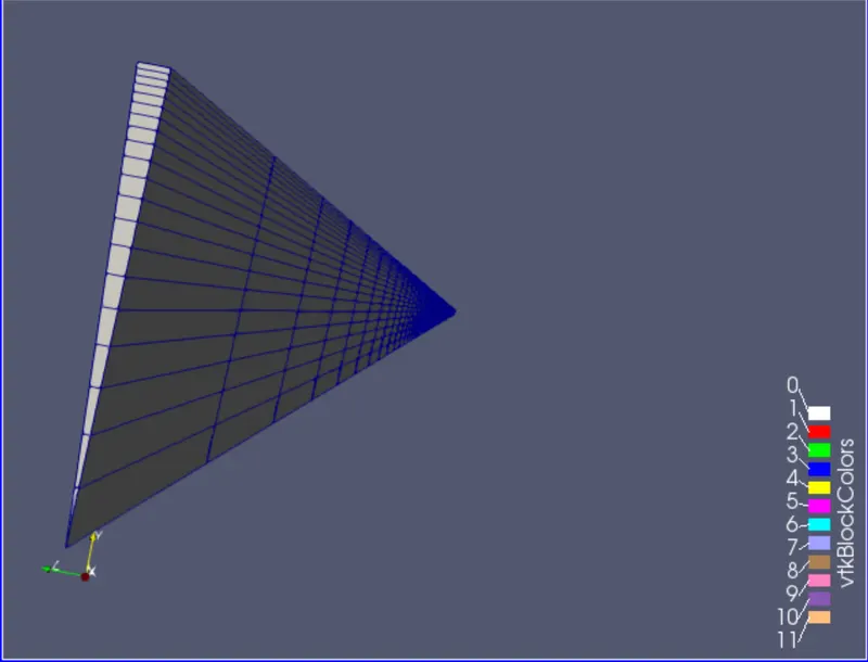
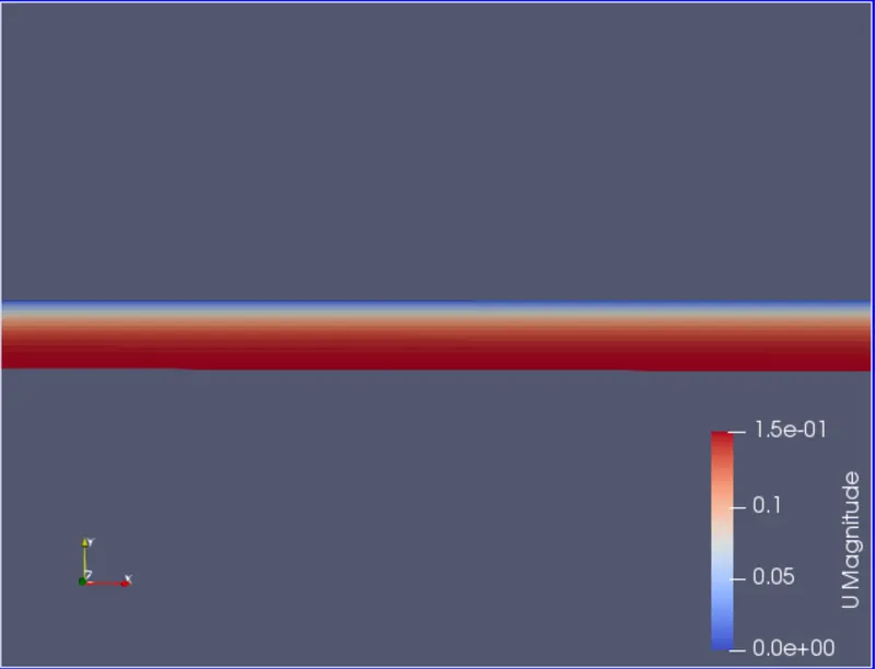
Velocity distibution:
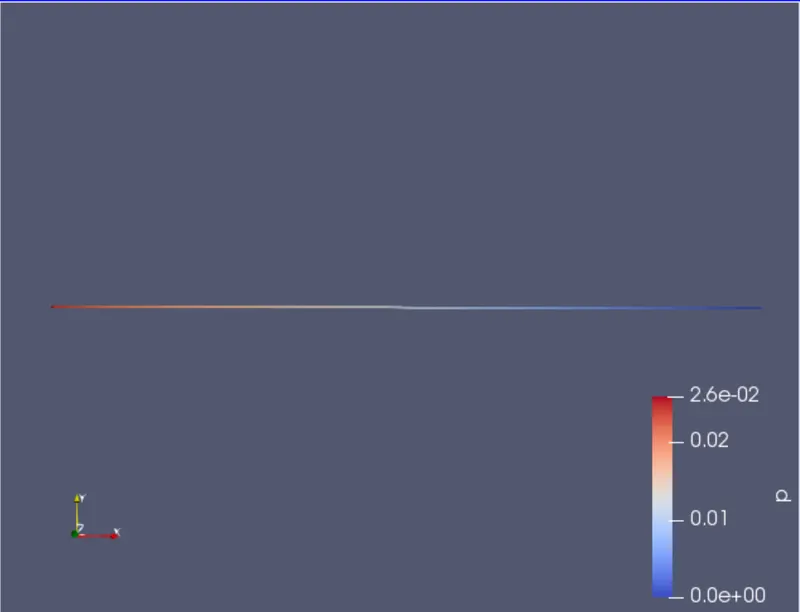
Pressure distribution:
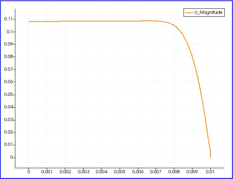
Velocity distribution at 0.025m:
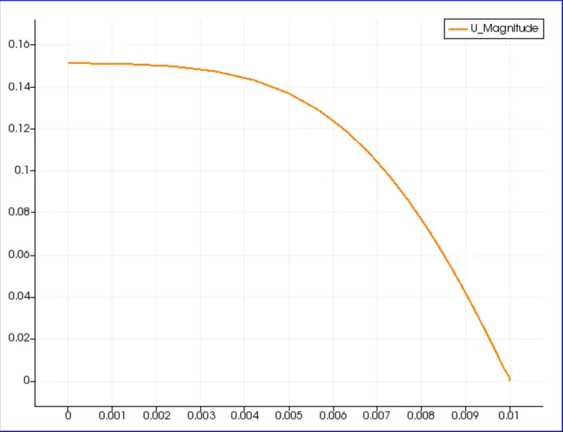
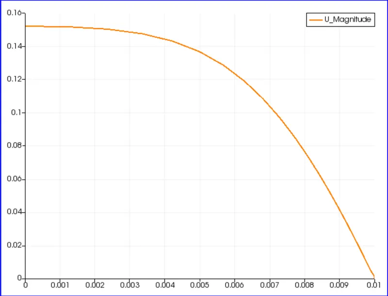
Velocity profile at 0.5m:
Velocity profile at 1m:
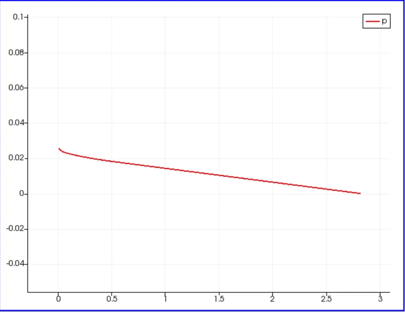
Pressure flow acroos the whole pipe:
Procedure explanation:
1.In openFoam ,choose the icoFoam solver in which we are working on incompressible laminar flow .
2.Copy the file from the solver in the run folder to simulate the file ,then we change the file geometry in blockMeshDict file .
3.Here we writ code for blockMeshDict file in matlab using file parsing and open it in OpenFoam and the boundary conditions for the simulatin are set in the Velocity and Pressure file and the Transport properties and controlDict file are suitably changed according to the flow .
4.After all the changes the blockMesh and checkMesh command are run to find the correctness of the geometry and the mesh and the solver icoFoam is run to simulate the geometry.
Post processing:
1.After opening paraview select apply to generate the geometry.
2.Press on the play button to post procees to end time.
3.Select the plot over line command and plot velocity magnitude and pressure with respect to the radial distance.
4.Write asuitable code in Matlab to calculate shear stress and plot graph for shear stress.
Matlab code for Shear stress:
close all
clear all
clc

D=0.02;
R=D/2;
r=linspace(-0.01,0.01,1000);
Re=2100;
mu=8.9e-4;
rho=1000;
V=(Re*mu)/(rho*D);
u_max=2*V;
for i=1:length(r)
    Tau(i)=(2*mu*u_max*abs(r(i)))/(R^2);
end
figure(1)
plot(r,Tau)
xlabel('Radial distance in m')
ylabel('Shear stress(Tau) in N/m^2')
title(sprintf('change in shear stress for fully developed flow at x=2.82m with radial distance'))
grid minor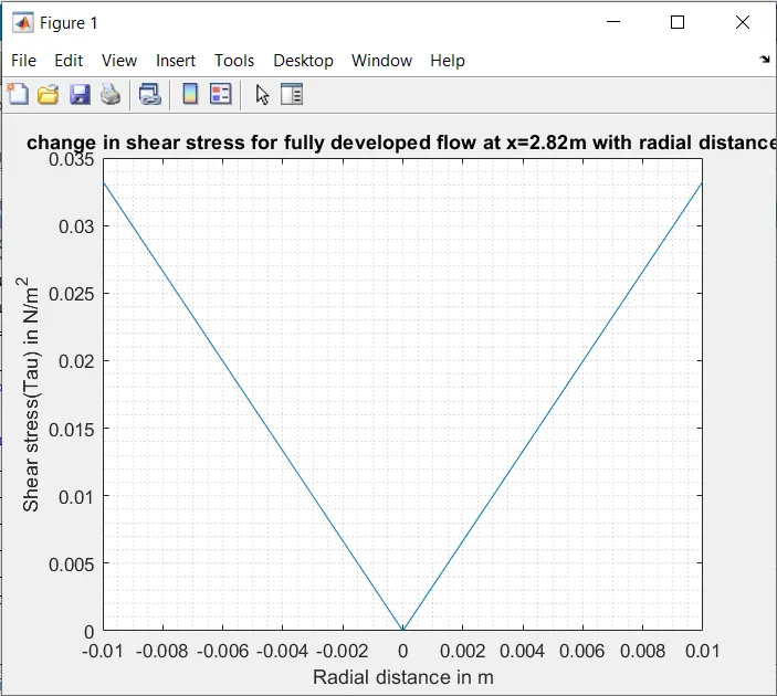
As we can see the shear stress increases along the radius i.e shear stress is 0 at centre of the pipe and its maximum at the walls.