Week 9 - FVM Literature Review

Finite Volume method:

• FVM is amethod for representing and evaluvating the partial differential equations in the form of algebraic equation , similar to FDM and FEM the values are calculated at discrete places.
• In the finite volume method, volume integrals in a partial differential equation that contain a divergence term are converted to surface integrals, using the Gauss divergence theorem.
• These terms are then evaluated as fluxes at the surfaces of each finite volume. Because the flux entering a given volume is identical to that leaving the adjacent volume, these methods are conservative.
• Another advantage of the finite volume method is that it is easily formulated to allow for unstructured meshes.

Steps in Finite volume discretization:

• Write the governing equations in integral form
• Apply Gauss divergence theorem.
• Come up with suitable flux terms.

Consider the 1D steady state heat equation

`del/(delx)(alpha(delt)/(delx))+S=0`

where S is the source term and `(delt)/(delx)` is the time gradient along x direction `alpha` is thermal diffusivity

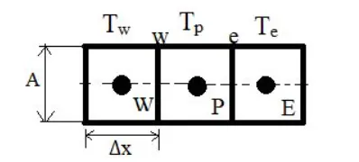
The governing equation is valid at every point in the domain which means it is valid in the entire control volume

Multiply the governing equation by dv and integratig it

`int(del/(delx)(alpha(delt)/(delx))+S)dv=0`

`intdel/(delx)(alpha(delt)/(delx))dv+intSdv=0`

dv= A*dx

`intdel/(delx)(alpha(delt)/(delx))A*dx+intSdv=0`

`[alpha A((delt)/(delx))]_w^e +s dv =0`

here s is the average value of source term

`alpha_e A((delt)/(delx_e))- alpha_w A((delT)/(delx_w)) +sdv=0`

heat flux (out )- heat flux(in)+ source term =0

Types of schemes:

1.Gradient scheme

For calculating the temperature gradient at east face we use neighbouring point temperature to numerically represent the temperature gradient this is called gradient scheme.

2.Interpolation schemes in FVM:

Interpolation is the process to estimate the values at unknown points by using the points with known values and sample points on either sides of the unknown point.In FVM the interpolation scheme is used to find the values of volume integrals required at the points other than the nodes.

the different schemes are

1. Upwind Interpolation scheme
2. Linear Interpolation scheme
3. Quadratic Upwind Interpolation scheme
4. Hybrid Interpolation scheme
5. Total variation dimnishing scheme
6. Essentially non-oscillatory interpolation scheme

Upwind Interpolation scheme

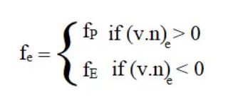
The upwind schemes attempt to discretize hyperbolic partial differential equations by using differencing biased in the direction determined by the sign of the characteristic speeds.The upwind interpolation scheme is essentially used for convection dominated problems and velocity at given point and direction of that which determines the variables used in the interpolation process.

The upwind interpolation of the variable f facing at east is given below

Linear interpolation scheme:

It is the simplest and most widely used method odf interpolation

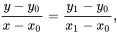
If the two known points are given by the coordinates and , the linear interpolant is the straight line between these points. For a value x in the interval, the value y along the straight line is given from the equation of slopes

Linear interpolation is often used to approximate a value of some function f using two known values of that function at other points. The error of this approximation is defined as

where p denotes the linear interpolation polynomial defined above:

for 1D heat conduction

`f_e=f_E+lambda_e +f_p(1-lambda_e)` where `lambda_e=(x_e-x_p)/(x_E-x_p)`

Quadratic upwind interpolation Scheme:

It is a higher-order differencing scheme that considers a three-point upstream weighted quadratic interpolation for the cell face values.

QUICK does take the second order derivative into account, but ignores the third order derivative hence this is considered third order accurate.

This scheme is used to solve convection diffusion equations using second order central difference for the diffusion term and for the convection term the scheme is third order accurate in space and first order accurate in time. QUICK is most appropriate for steady flow or quasi-steady highly convective elliptic flow.

In this case we have to approximate the value of variable at CV face centre by quadratic interpolation of the values at three nearest computational nodes

`f_e=f_U+g_1(f_D-f_u)+g_2(f_(UU)-f_u)`

`g_1=((x_e-x_U)(x_e-x_(UU)))/((x_D-x_U)(x_D-x_(UU))`

`g_2=((x_e-x_U)(x_e-x_U))/((x_(UU)-x_D)(x_(UU)-x_U)`

Hybrid Interpolation scheme:

It is the combination of upwind interpolation scheme and central difference scheme based on the local peclet number.The general partial differential equation is as follows

`f_e=lambdaf_(CDS)+(1-lambda)f_(UDS)`

Total variation dimnishing scheme:

`f_e=f_p+1/2psi(r)(f_E-f_p)`

where `psi`is the flux limiter and r is the specified condition which depends on local flow conditions.

Flux Limiters:

Flux limiters are employed in high resolution schemes,which are numerical systems for solving problems in science and engineering , especially fluid dynamics that are described by partial differential equations.They are employed in high resolution scheme to eliminate oscillations ,shocks, discontinuities and rapid changes in the solution domain that would otherwise occur with higher order spatial discretization schemes.

`(du_i)/(dt)+1/(dx_i)[F(u_(i+1/2))-F(u_(i-1/2))]=0`

`F(u_(i+1/2))= f_(i+1/2)^(low) - phi(r_i)(f_(i+1/2)^(low)-f_(i+1/2)^(high))`

`F(u_(i-1/2))= f_(i-1/2)^(low) - phi(r_i-1)(f_(i-1/2)^(low)-f_(i-1/2)^(high))`

where `f^(low)` is low resolution flux

`f^(high)` is high resolution flux

`phi(r)` is flux limiter function

r represents ratio of successive gradient on the solution mesh

Finite difference method:

A finite difference method (FDM) discretization is based upon the differential form of the PDE to be solved. Each derivative is replaced with an approximate difference formula (that can generally be derived from a Taylor series expansion). The computational domain is usually divided into hexahedral cells (the grid), and the solution will be obtained at each nodal point. The FDM is easiest to understand when the physical grid is Cartesian, but through the use of curvilinear transforms the method can be extended to domains that are not easily represented by brick-shaped elements. The discretization results in a system of equation of the variable at nodal points, and once a solution is found, then we have a discrete representation of the solution.

Finite element method:

A finite element method (FEM) discretization is based upon a piecewise representation of the solution in terms of specified basis functions. The computational domain is divided up into smaller domains (finite elements) and the solution in each element is constructed from the basis functions. The actual equations that are solved are typically obtained by restating the conservation equation in weak form: the field variables are written in terms of the basis functions, the equation is multiplied by appropriate test functions, and then integrated over an element. Since the FEM solution is in terms of specific basis functions, a great deal more is known about the solution than for either FDM or FVM. This can be a double-edged sword, as the choice of basis functions is very important and boundary conditions may be more difficult to formulate. Again, a system of equations is obtained (usually for nodal values) that must be solved to obtain a solution.

Difference between the three methods:

Comparison of the three methods is difficult, primarily due to the many variations of all three methods. FVM and FDM provide discrete solutions, while FEM provides a continuous (up to a point) solution. FVM and FDM are generally considered easier to program than FEM, but opinions vary on this point. FVM are generally expected to provide better conservation properties, but opinions vary on this point also.