Week 5.2 - Literature review: ODE Stability

Introduction:

In a system when a disturbance occurs, and if the system tends to minimize the error or disturbance then it is a stable system. But whereas, when the error or disturbance arises to continue and not decrease the system is said to be unstable.

In Numerical discretization, a small error appears during mathematical approximation.This error needs to be checked or solved for every iteration to maintain a stable solution.

A ODE can be solved by numerically various methods like Euler's Method and Range-Kutta Method.

Euler's Method:

The Euler method is a first-order method, which means that the local error (error per step) is proportional to the square of the step size, and the global error (error at a given time) is proportional to the step size.

In Euler's method, there are two method

1. Explicit method
2. Implicit method

The explicit method uses the system status from present to find the future status of the system.

The implicit method uses the system status from present and future to calculate the system future status. It uses backward differencing method

If y is a function y=f(x,t)

Explicit method is expressed as `y_(n+1) = y_n +hf(x_n,t_n)`.From the known state n we can calculate the future state n+1.

Implicit method is expressed as `y_n=y_(n-1) +hf(x_n,t_n)`. Here we use the state n and n-1 to calculate the current state n.

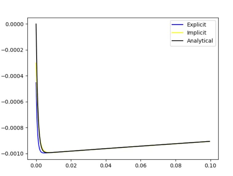
Codes are written for explicit , implicit method and analytical and plotted.

Code:

import numpy as np
import matplotlib.pyplot as plt
def explicit(total_t,dt):
		
	t=np.arange(0,total_t,dt)
	y=np.zeros(len(t))

	for i in range(0,len(t)):
		y[i]=y[i-1]+dt*(-1000*y[i-1] -np.exp(-t[i-1]))

	return [t,y]

def implicit(total_t,dt):
		
	t= np.arange(0,total_t,dt)
	y=np.zeros(len(t))

	for i in range(0,len(t)):
		y[i]=(y[i-1]-np.exp(-t[i-1])*dt)/(1+1000*dt)

	return [t,y]

def analytical(total_t,dt):
		
	t= np.arange(0,total_t,dt)
	y=np.zeros(len(t))

	for i in range(0,len(t)):
		y[i]=np.exp(-1000*t[i])*(1-np.exp(999*t[i]))/999

	return [t,y]

total_t = 0.1
dt=0.005
t,y_exp=explicit(total_t,dt)
t,y_imp=implicit(total_t,dt)
t,y_analy=analytical(total_t,dt)
plt.plot(t,y_exp,color='blue')
plt.plot(t,y_imp,color='yellow')
#plt.plot(t,y_analy,color='black')
#plt.legend(('Explicit','Implicit','Analytical'))
title=('Timestep:',dt)
plt.show()

Plot: (at dt = 0.0005s):

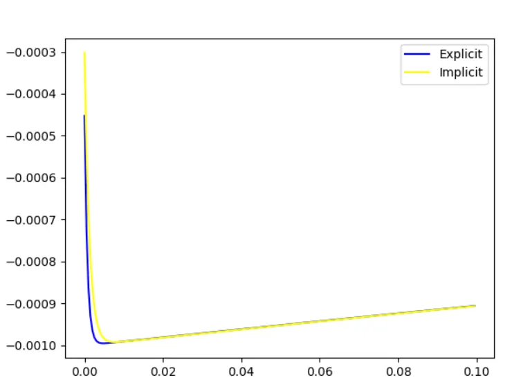
at dt= 0.005s:

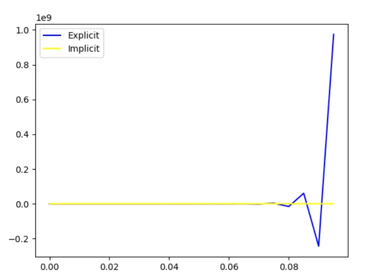
The problem arises due the larger value of dt.It can be seen that the explicit method results blows out while the implicit answer is a flat line.This can be clearly explained by the below comparison.

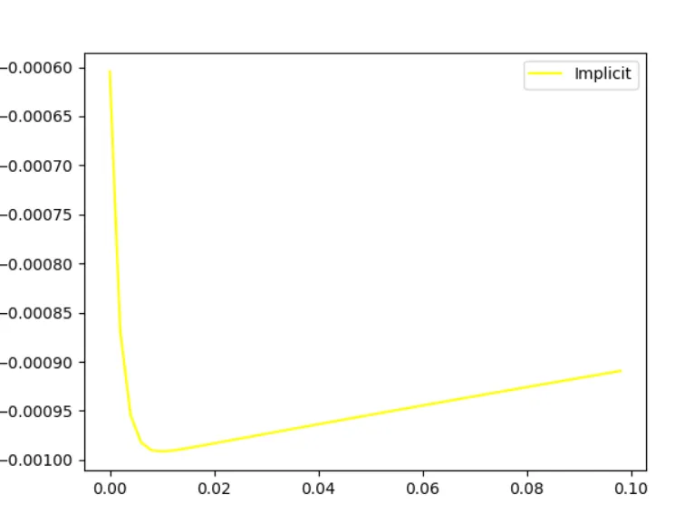
Implicit method (at dt =0.002s):

Explicit method at dt =0.002s:

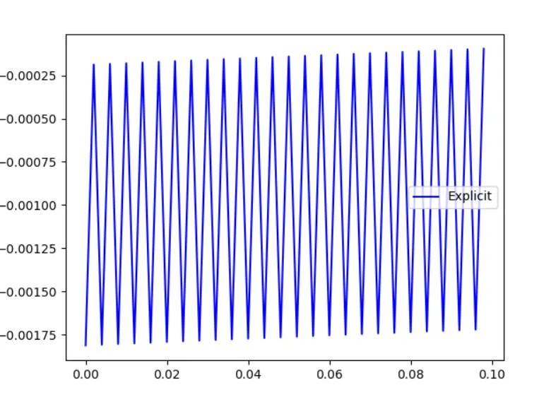
From the above results we can see that for a larger step dt the implicit method gives a stable solution whereas explicit method throws useless values.

Implicit ,Explicit and Anlytical solution at dt=0.0005s:

When does a ODE become unstable?

The implicit method calculates simulataneous equations to achieve the results so even when the dt value is increased it continues to give a result as it solves for full grid and each time step.

But in explicit method as the dt value gets larger the solution becomes unstable as it uses present and past values of the system to compute the future values.

How does stability affect engineering simulations?

Stability guarantees that the numerical method produces a bounded solution that converges with the exact solution of the differential equation.If the solution aren't bounded then it diverges from the exact solution , can't be derived for a particular simulation.

Can stability condition be derived for all types of problems?

A neutrally stable scheme is one which the error remains constant as it uses forward differencing. Implicit schemes does not have to satisfy stability conditions and are unconditionally stable as they use backward differencing.But it is computationally expensive as it takes a large amount of space,as it uses the n+1 time level on the lhs to compute the equation.

So we can solve a equation using implicit scheme using proper selection of the time step.

The Courant–Friedrichs–Lewy or CFL condition is a condition for the stability of unstable numerical methods that model convection or wave phenomena.

It follows from the numerical diffusion coefficient discussion, that for any explicit simple linear convection problem, the Courant number must be equal or smaller than 1, otherwise, the numerical viscosity would be negative and results in unstable solution.