CHT Analysis on Exhaust manifold

# Abstract:
Conjugate Heat Transfer (CHT) analysis is carried out for the exhaust manifold of an inline `4` cylinder engine. Heat transfer coefficient (HTC) on the outer surface of the exhaust is taken as `20` `W//m^2 K`, the inlet temperature of exhaust gases as `700` K, ambient temperature as `300` K & inflow velocity of `5` `m//s`. Steady-state simulations are performed for Reynolds number of `1.1351` x `10^(4)` and HTC on the fluid-solid interface is computed in steady-state conditions assuming roughness of `6` `mum`. Grid dependency test is carried out. Commercially available CFD tool ANSYS® Fluent® 2021 R2 Student version is used.

# Introduction:

Exhaust manifold
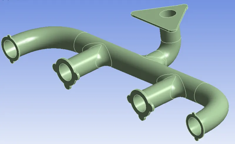
The exhaust manifold of an inline four-cylinder engine is shown below. It has an outlet which collects exhaust gases from the four inlets and delivers them to the exhaust pipe. There are also flanges for securing the component to the engine & exhaust pipe, the flanges are assumed to have adiabatic outer walls.

CHT Analysis
In many applications it is common for fluid flows to interact physically (& sometimes even chemically) with solid surfaces. Heat transfer between fluid-solid interface is the most common interaction that can induce changes in temperature, pressure, phase, etc in the fluid with or without the intent of the design.

Hence Conjugate Heat Transfer (CHT) analysis is carried out for exhaust manifold simulations as well which allows for the simulation of heat transfer between solid and fluid domains by exchanging thermal energy at the interfaces between them.

Typical applications of CHT analysis are the simulation of heat exchangers, cooling of electronic equipment, and general-purpose cooling and heating systems.

# Numerical model:
Turbulence model
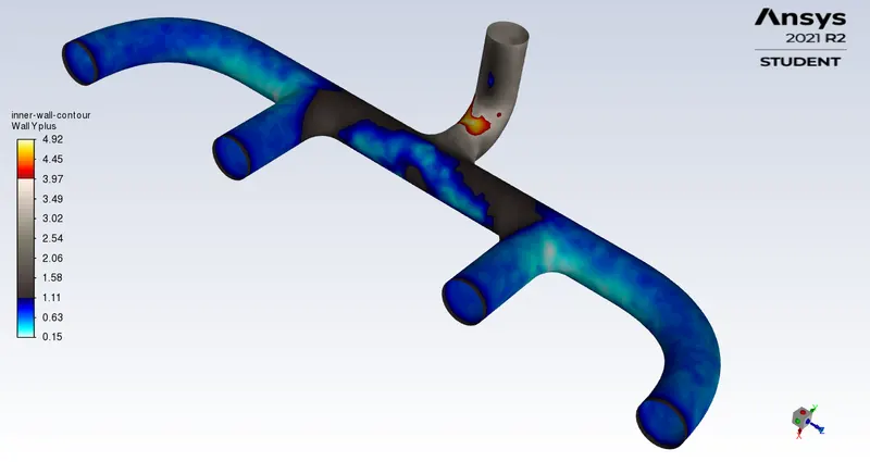
The flow will be attached throughout the domain hence for reduced computational effort RANS based SST `k-omega` turbulence model is used with standard wall functions for near-wall modeling. The `y^+` is chosen as `0.9` and along the model walls the `y^+` values are checked after a few initial iterations and also during post-processing so that they fall in the desired range of `y^+<5`.

Solution method
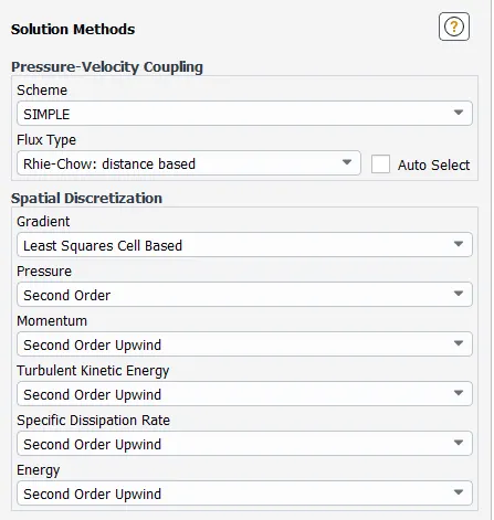
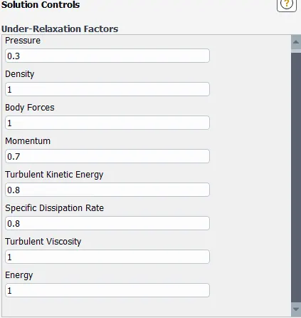
The solution procedure is iterative and is based on SIMPLE scheme for Pressure-Velocity coupling. The discretization is `2^(nd)` order for pressure and `2^(nd)` order upwind for other variables. The gradient is computed using the Least-squares cell-based method. Commercially available CFD tool ANSYS® Fluent® 2021 R2 Student version is used which has a limit of 512,000 cells in the mesh.

# Computational domain:
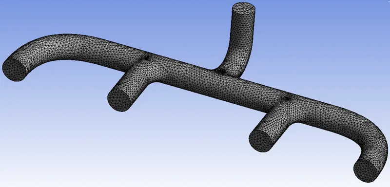
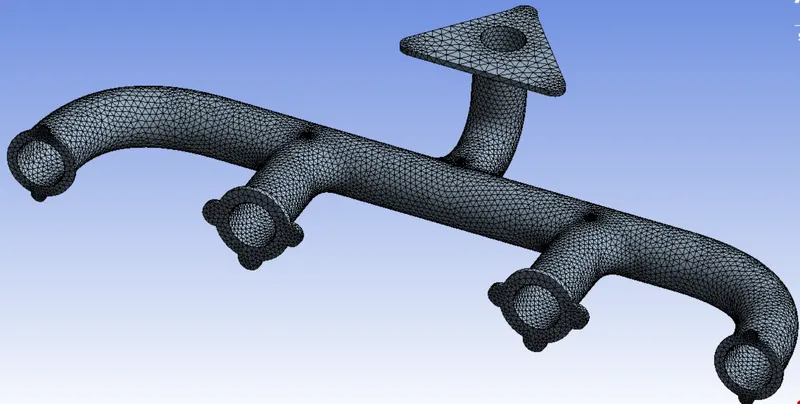
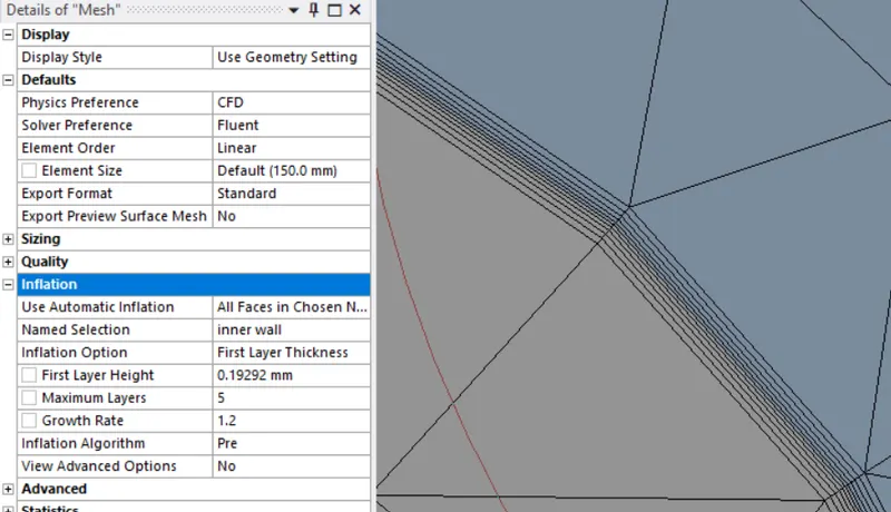
The computational domain is divided into the fluid domain and the solid domain. The common surface of the interface between them is the shared topology so as to allow perfect mesh connectivity across the entire domain. The fluid domain is meshed more finely than the solid domain. Inflation layers are added on the surface of the interface so that information travels smoothly and accurately.

# Boundary Conditions:
Boundary conditions were set as 'velocity inlet' at inlet faces with velocity normal to surface as `5` `m//s` at `700` K, 'pressure outlet' at outlet face, 'wall' on the fluid-solid interface (named inner wall) with no-slip, ‘wall’ with constant HTC of `20` `W//m^2 K` & ambient temp. `300` K on surface named ‘outer-wall-convection`.

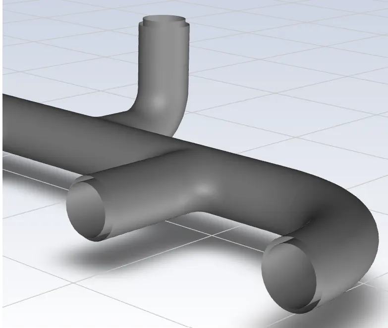
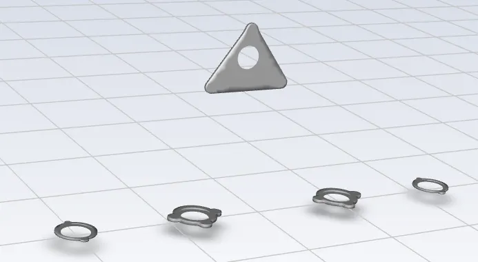
The remaining surfaces were set as ‘wall’ with adiabatic conditions.

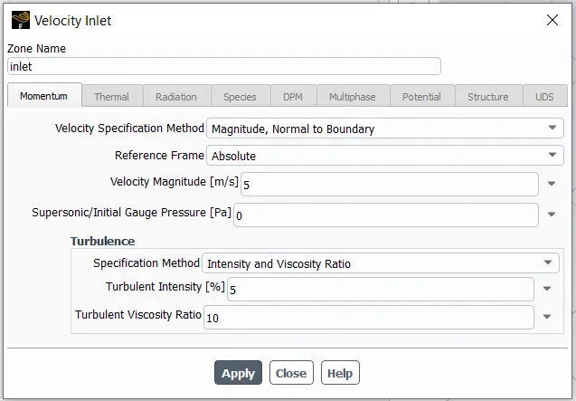
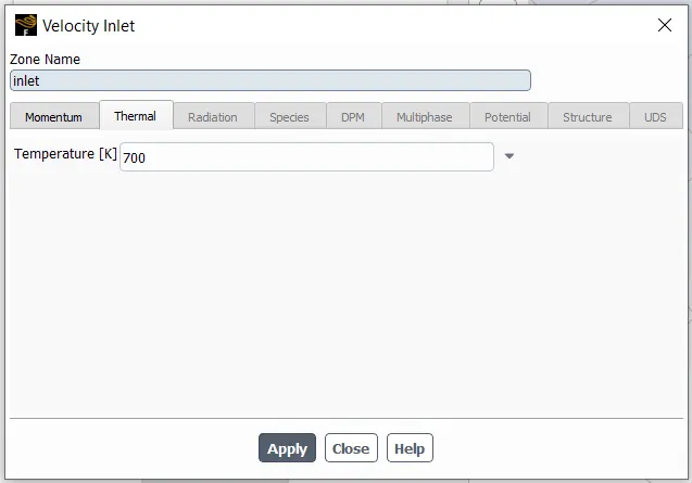
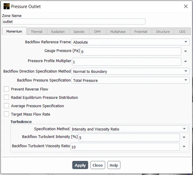
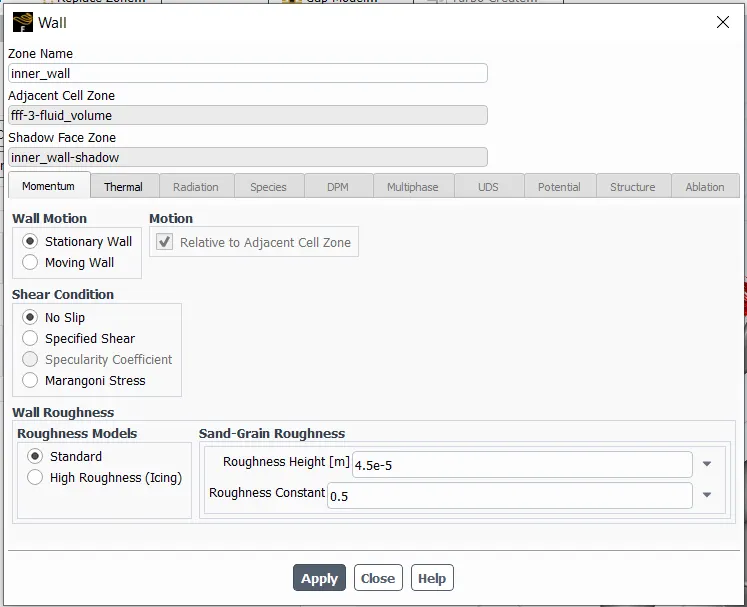
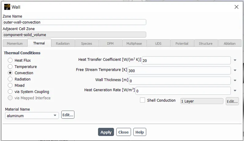
Figure: Boundary conditions

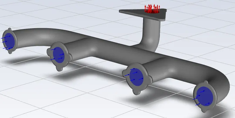
(a) inlets and outlet (b) Inner and outer walls

(c) Walls set to adiabatic conditons

Figure: Wall geometry

# Solver settings:

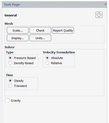
• Since the Mach no. `(5//sqrt(gamma R T) = 0.0943)` of flow is less than `0.3` pressure based steady-state solver is used with pressure-velocity coupling using SIMPLE algorithm. Least squares cell-based method is used for computing gradients.
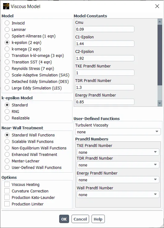
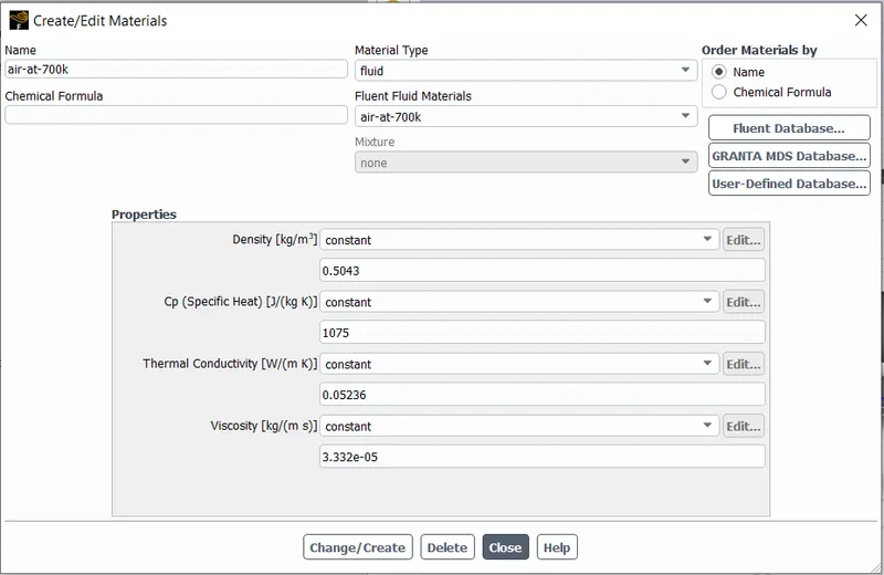
• SST `k-omega` turbulence model was selected with `y^+` of `0.9` and properties of air at `700` K were set using create fluid option.
• All simulations were carried out for `500` iterations after hybrid initialization.

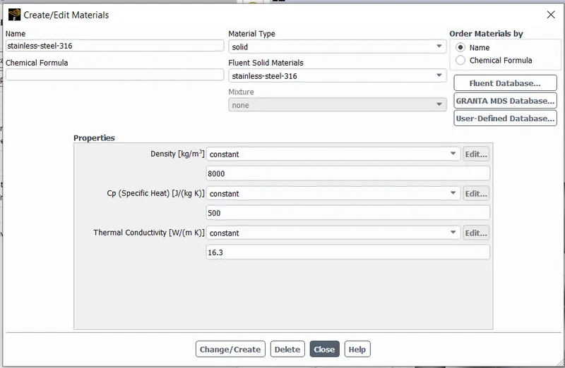
• 316 Stainless Steel is used as material for the component [1], the roughness height of S.S. (new) is `45``mum`[2] and relative roughness is `3` x `10^(-4)`. It is assumed to have uniform roughness so, the roughness constant is taken as `0.5`.

Calculating first cell centre distance for inflation layer:
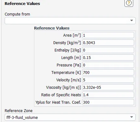
For air at `700 K`, [2]
`" "rho = 0.5043` `kg//m^3`
`" "mu = 3.332` x `10^(-5)` `kg//m s`
`" "nu = 6.607` x `10^(-5)` `m^2//s`

Also,
`" "U_oo = 5` `m//s`
`" "D = "Hydraulic diametre" = 0.150` `m`
`" "epsi = "pipe roughness" = 6` x `10^(-6)` `m` [3]

Reynolds number,
`Re = (rho U_oo D)/mu = 1.1351` x `10^(4)`

The Colebrook-White equation was solved by iteration to calculate skin friction coefficient `lambda//4` (Darcy Friction factor/4),
`" "sqrt(1/ lambda) = -2 log [2.51/((Re sqrt(lambda))) + ((epsi//D))/3.72] ` [4]
`" "therefore lambda = 0.0304`
`" "therefore C_f = lambda//4 = 0.0076`

Wall shear stress,
`" "tau_w = C_f""(1/2rho U_(oo)^2) = 0.04791` `N//m^2`
Friction velocity,
`" "u_r = sqrt(tau_w/rho)= 0.30822`
First cell center (or first layer thickness) for `y^+` of 0.9,
`" "y = (y^(+)nu)/u_r = 2.14359` x `10^(-4)` m `= 0.214359` mm

# Baseline simulation results:

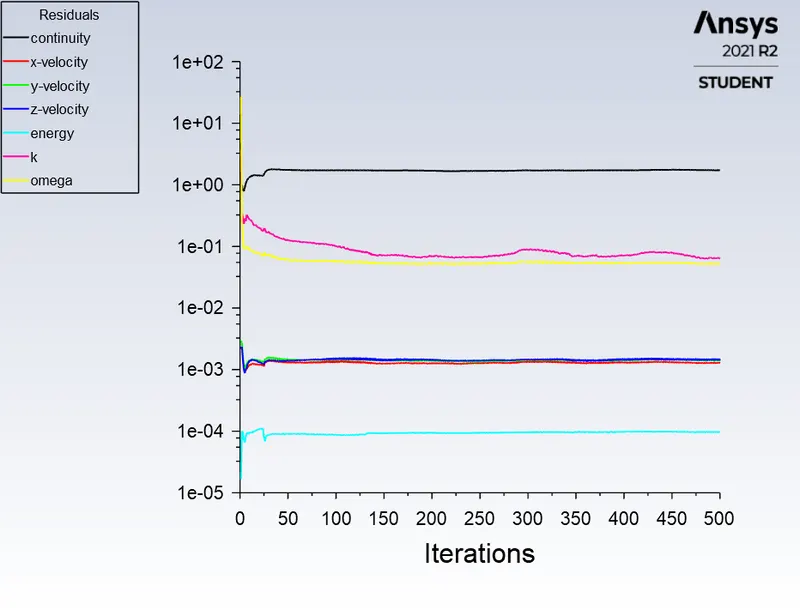
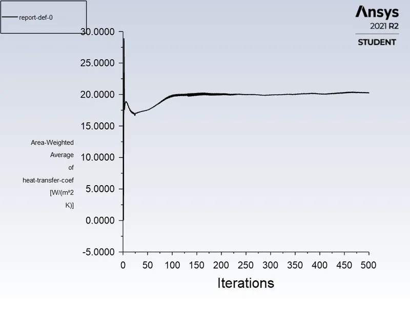
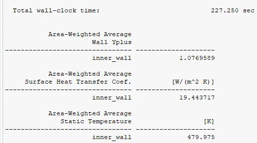
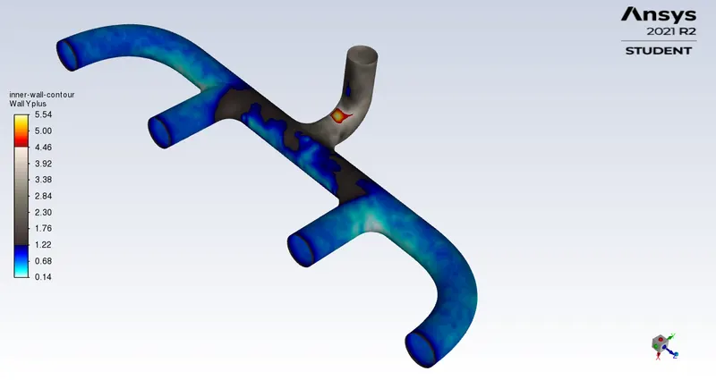
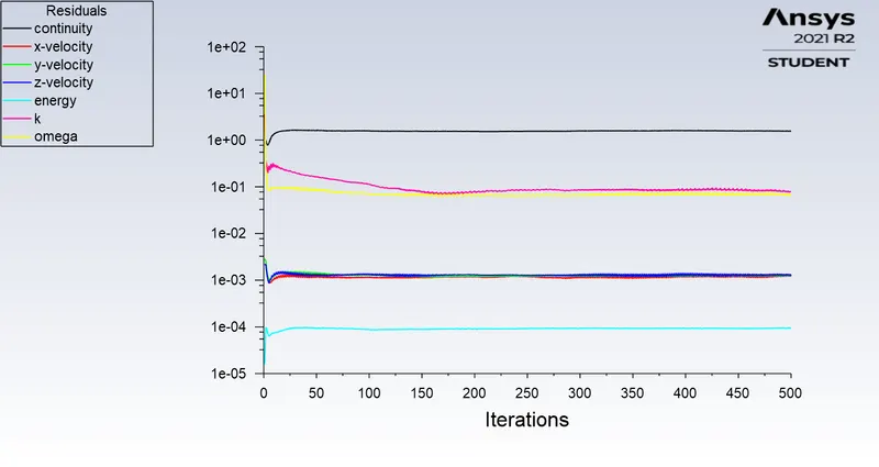
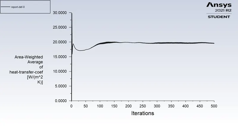
The convergence plots and `y^+` values over the inner wall are shown. The convergence plots show a repeated pattern with small fluctuations hence we can say that the results have converged. Also, the mean value of `y^+` is near `1` over the entire inner wall surface so, the viscous sublayer is resolved sufficiently.

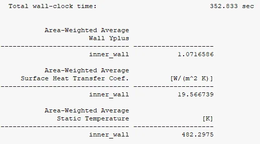
The area-weighted average values are computed over the inner wall surface.

REFINED RESULTS BELOW>

Convergence plots

`y^+` value at steady state

# Grid dependency:

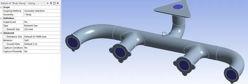
Multiple simulations were performed with increasing mesh refinement near the inner wall surface of the exhaust manifold and key results are tabulated below.

Mesh no.	Face sizing on 'inner wall' (mm)	no. of cells	Computation time (sec)	Area weighted average of `y^+` (on inner wall)	Area weighted average of HTC (`W//m^2 K`)	Percentage change in HTC
1	20	323,663	277.25	1.0769	19.4437	-
2	18	378,707	272.2	1.0575	19.1623	-1.45
3	16	463,563	245.726	1.0603	19.0194	-0.75
4	15.12	511,024	352.833	1.0717	19.5667	+2.88
				Average =	19.2980

We can see that the results vary less than `5%` we can say that mesh `1` is grid-independent and hence further refinement will only increase computation cost. However, a finer mesh allows for a smoother contour plot of variables of interest hence the results from the last refined mesh `4` was used for post-processing the results. The results will be very similar even with mesh `1`.

Since the HTC values show a small variation, we can take an average value of `19.298` `W//m^2 K`.

# Post processing:

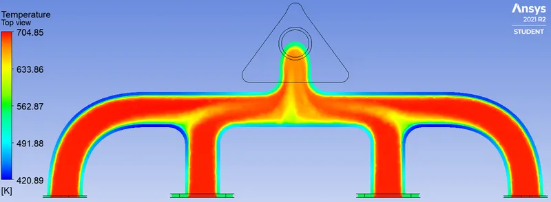
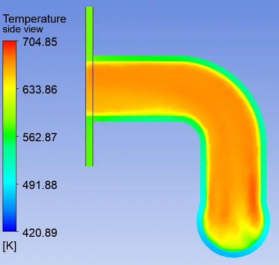
Temperature Contours

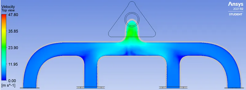
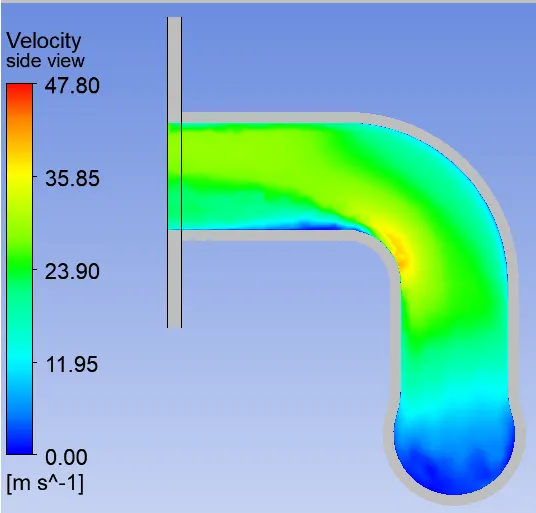
Velocity contours

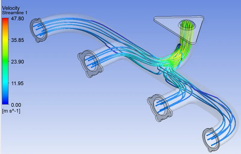
Velocity streamlines

Computed values

# Validation:

Gnielinski Equation [5]
The Gnielinski Equation (for transition & turbulent flow) is an explicit function for calculating the Nusselt number. It is a bit more complex than Dittus-Boelter and Sieder-Tate equations but is also more accurate. This equation is valid for tubes over a large Reynolds number range including the transition region. The equation is:

`Nu_D= ((lambda//8)(Re-1000)(Pr))/(1+12.7((lambda//8)^(1//2))((Pr)^(2//3)-1))`

Where,

`D` is the inside diameter of the circular duct
`Pr` is the Prandtl number
`lambda` is Darcy friction factor

The Gnielinski Equation is valid for:-

`0.6<=Pr<=2000`

`3000<=Re_D<=5` x `10^6`

In our case,

`Pr = (muc_p)/k = (3.332"x"10^(-5)*1075)/(5.236"x"10^(-2)) = 0.6841`

`Re_D = 11351`

Therefore the analytical value is,

`Nu_D= ((0.0304//8)(11351-1000)(0.6841))/(1+12.7((0.0304//8)^(1//2))((0.6841)^(2//3)-1)) = 32.618`

`therefore h = ((Nu_D)(k))/((L_c)) = 11.38` `W//m^2 K`

The numerical value is `19.298` `W//m^2 K`.

# Conclusion:

The analytical & numerical values of HTC differ significantly however it is to be noted that the Gnielinski equation is valid for a straight pipe section with a fully developed thermal boundary layer hence this degree of disagreement between the two values is expected.

There is no better way to judge how accurate our HTC prediction is other than actual experimentation because the component geometry is complex and HTC is very difficult to analyze mathematically as it depends on a lot of factors like flow characteristics, fluid properties, geometry, surface orientation & roughness.

The accuracy of HTC predictions using CFD also depends on:-

• how accurately real geometry is represented by modeled geometry.
• The mesh refinement, quality & connectivity.
• Proper resolution of the boundary layer and turbulence model used.
• Selecting
• Deviation of actual operating conditions from the ones assumed in the numerical model.

The simulations carried out show that the solution becomes mesh independent after `323,663` cell count with face sizing of `20` `mm`. The procedure shown here hence be used to obtain HTC through the inner surface of the exhaust manifold in a reasonable time for creating preliminary designs.

References:

[1] The material used for exhaust manifold,https://dergipark.org.tr/tr/download/article-file/318350

[2] Roughness of commercial steel,https://thermopedia.com/content/789/

[3] Properties of dry air at 700k,https://www.engineeringtoolbox.com/dry-air-properties-d_973.html

[4] Colebrook-White equation and friction factor from the moody diagram,https://thermopedia.com/content/789/

[5] V. Gnielinski, “New Equations for Heat and Mass Transfer in Turbulent Pipe and Channel Flow,” International Chemical Engineering, Vol. 16, No. 2, 1976, pp. 359-68.