External flow simulation over an Ahmed body.

# Abstract:

The aerodynamic behavior of Ahmed body is investigated numerically and the coefficient of drag is validated with experiments from literature. Simulations use a slant angle of `25^@`, yawing angle of `0^@`, and Reynolds number of `1.664` x `10^(6)`. Grid dependency test is carried out and results agree fairly with data from the available literature. Commercially available CFD tool ANSYS® Fluent® 2021 R2 Student is used.

# Introduction:

The Ahmed body

Ahmed body was developed by S.R. Ahmed & presented in his research paper “Some Salient Features of the Time-Averaged Ground Vehicle Wake” in 1984. This body is used as a generic car body because it captures all the essential flow features around an automobile and is easy to model. The simple model makes meshing easier, reduces the computational power required and the time taken to run the simulations.

Hence the body is widely used by researchers & engineers to validate their numerical model or CFD codes and sometimes without even wind tunnel testing as vast experimental data is already available (for different scale models of Ahmed body) from validation studies over the years.

The geometrical shape of Ahmed body is shown in figure(1). Despite the simplicity of this body, it represents the aerodynamic properties of a vehicle, especially in the rear part.

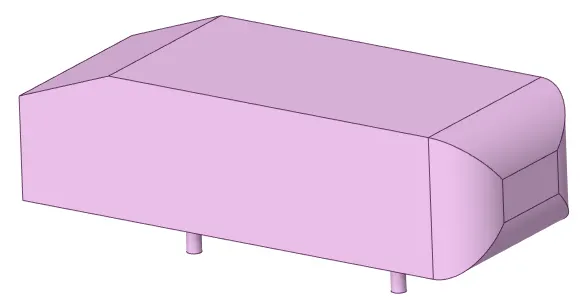
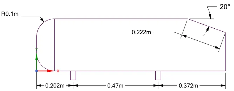
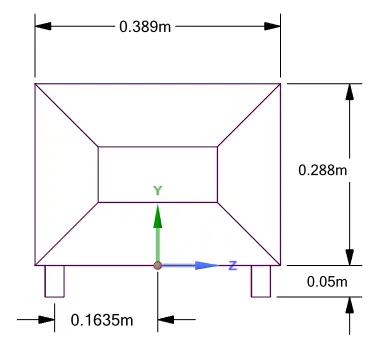
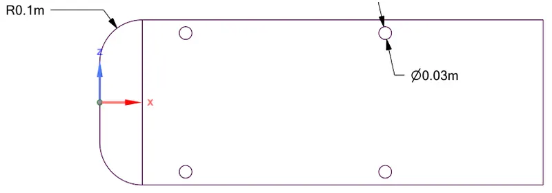
Figure (1): Ahmed body geometry

Negative pressure in the wake region

The flow separation due to an adverse pressure gradient in the rear end of Ahmed body generates a wake which is nothing but vortices that create negative pressure.

Point of separation

Separation takes place due to excessive momentum loss near the wall in a boundary layer trying to move downstream against increasing pressure gradient which is called adverse pressure gradient.

It is important that flow remains attached along the length of a vehicle (here Ahmed body) as far as possible because flow separation induces pressure drag leading to loss of kinetic energy of the vehicle. So the point of separation should be as far as possible near the rear end of the vehicle.

# Numerical Model:

Turbulence model
For reduced computational effort realizable `k-epsilon` turbulence model is used with standard wall functions for near-wall modeling. The `y^+` is chosen as 30 and along the model walls the `y^+` values are checked during post-processing so that they fall in the desired range of 30<y^+<300.

`k-epsilon` model is suitable for high Reynolds number flows and gives lower computation times.

Solution method
The solution procedure is iterative and is based on SIMPLE scheme for Pressure-Velocity coupling. The discretization is 2^(nd) order for pressure and 2^(nd) order upwind for other variables. The gradient is computed using the Least-squares cell-based method. Commercially available CFD tool ANSYS® Fluent® 2021 R2 Student version is used which has a limit of 512,000 cells in the mesh.

# Computational domain:
The computational domain consists of two bounding boxes. The size of the above computational domain can be reduced considering the symmetrical nature of flow around the longitudinal centroidal plane of Ahmed body. For this, the domain is split into two halves and the other half is removed. This domain can be meshed more finely and with reduced computation cost.

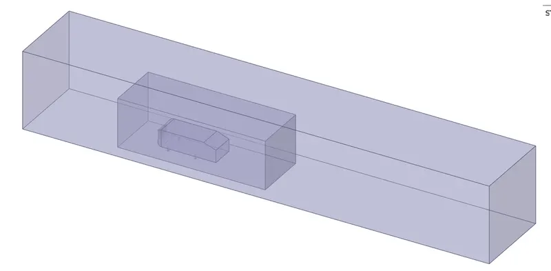
(a) Full computational domain

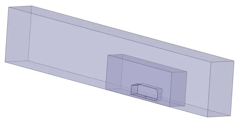
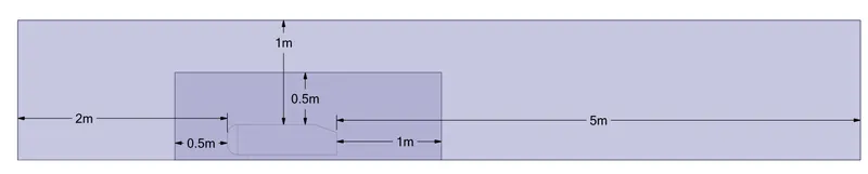
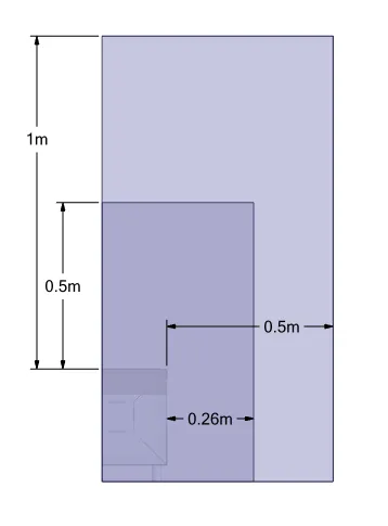
(b) Reduced computational domain

Figure (2): Computational Domain

The outer box (representing wind tunnel) is meshed with a bit coarse, higher quality hexahedral cells as flow variation is low in this region and the inner bounding box has finer trigonal mesh for capturing flow around & in wake of the body.

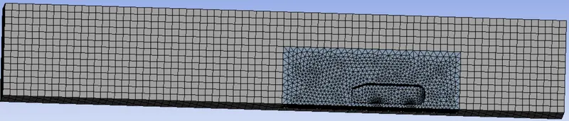
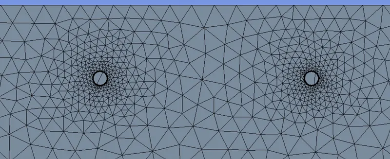
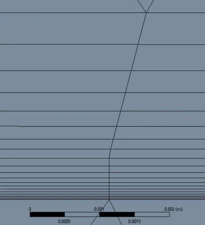
Figure (3): Domain Meshing

Calculating Y+ and inflation layer thickness:
For air at `300 k`,
`" "rho = 1.177" "kg//m^3`
`" "mu = 1.846` x `10^(-5)" "kg//m s`
`" "nu = 1.568` x `10^(-5)" "m^2//s`
Also,
`" "U_(infty) = 25" "m//s`
`" "L = "Characteristic length" = 1.044" "m`
Reynolds number,
`" "Re = (rho U_(infty) L)/mu = 1.664` x `10^(6)`

Skin friction coefficient using Prandtl’s 1/7 th power law,
`" "C_f = 0.027Re_d^((-1//7)) = 3.488` x `10^(-3)`
Wall shear stress,
`" "tau_w = C_f``(1/2rho U_(infty)^2) = 1.283" "N//m^2`
Friction velocity,
`" "u_r = sqrt(tau_w/rho)= 1.0441`
First cell center (or first layer thickness) for `y^+` of 1,
`" "y = (y^+ nu)/u_r = 1.5` x `10^(-5)" "m = 1.5` x `10^(-2)" "mm`

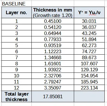
The above formula is utilized in an excel file to obtain `y^+` values for different layers. The baseline simulation will use a total boundary layer thickness of around 17 mm.

# Solver settings:

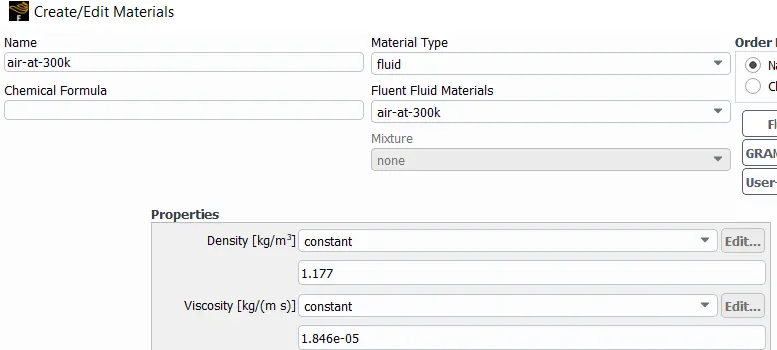
A pressure-based steady-state solver is used. `k-epsilon` turbulence model was selected and properties of air at 300k were set using create fluid option. Boundary conditions were set as 'velocity inlet' at inlet face with velocity normal to surface as `25" "m//s`, 'pressure outlet' at outlet face, 'wall' at car body with no-slip and 'symmetry' on remaining surfaces.

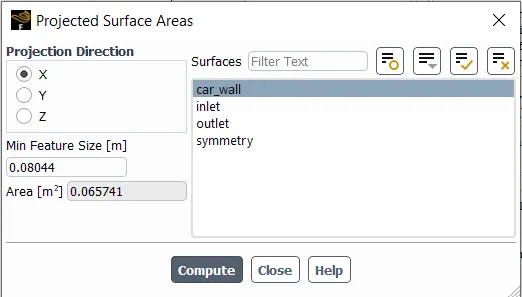
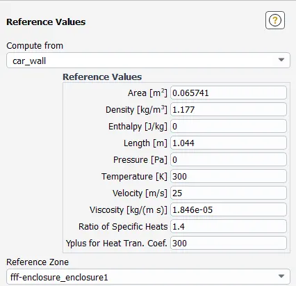
Reference values were set for the temperature of 300k along with the computed projected area of the car body along the x-axis. SIMPLE scheme is used for Pressure-Velocity coupling. All simulations were carried out for 350 iterations after hybrid initialization.

# Baseline simulation:

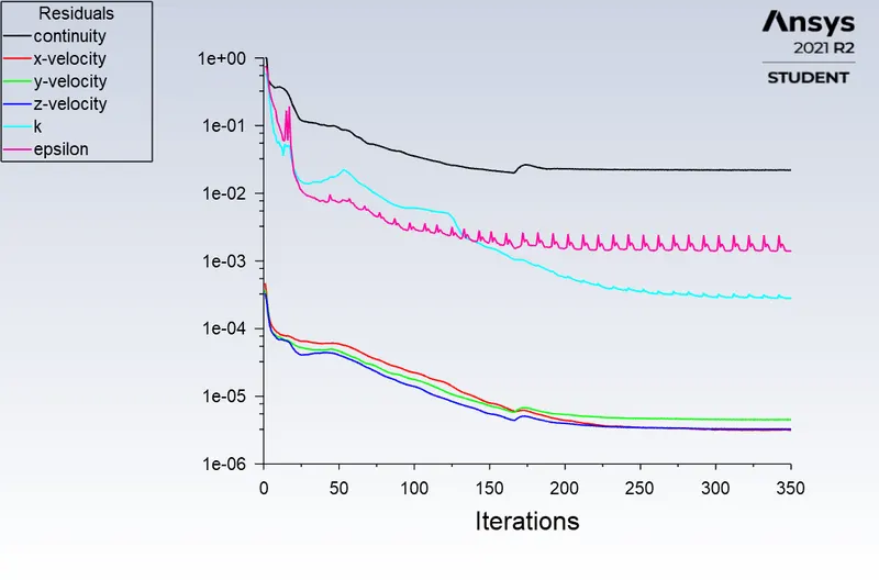
The results from the baseline simulation are shown below. The velocity contour on the midplane of Ahmed body can be seen below with mesh lines. It is similar to contours seen in Ahmed body simulations hence we can say that the physics of the phenomenon is captured but further mesh refinement is needed so that the solution is mesh independent and accurate.

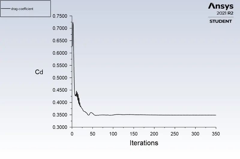
(a) Convergence plots

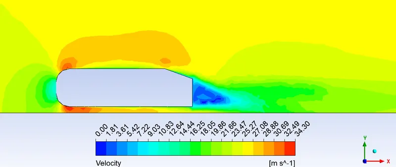
(b) Velocity contour

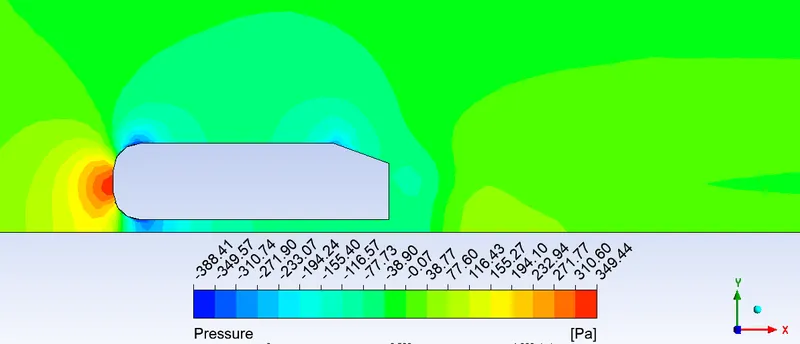
(c) Pressure contour

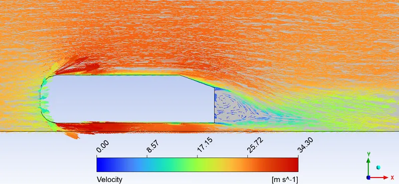
(d) Velocity vector plot

Figure (4): Baseline simulation results

# Results & Inferences:

The results from mesh refinement are summarised in the table below. For each refinement, the mesh in the inner bounding box was made finer while the mesh in the outer bounding box remained the same.

Case	Finer mesh size	Cells	Coefficient of drag `(C_D)`	Coefficient of lift `(C_L)`	Percentage Change
					`C_D`	`C_L`
Baseline	`5` x `10^(-2)`	`104,381`	`0.3491`	`0.2360`	`-`	`-`
Refinement 1	`3` x `10^(-2)`	`283,328`	`0.2998`	`0.2803`	`-14.12`	`18.77`
Refinement 2	`2.5` x `10^(-2)`	`443,273`	`0.3135`	`0.2450`	`4.55`	`-12.60`
Refinement 3	`2.37` x `10^(-2)`	`508,907`	`0.2936`	`0.2811`	`-6.35`	`14.73`

It can be seen that the percentage change in drag coefficient is around 6% for the most refined case which is ok. The post-processing results for this refined case (Refinement 3) are shown below.

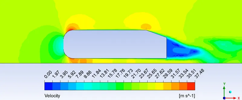
(a) Velocity contour

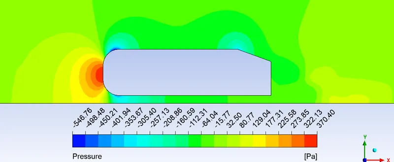
(b) Pressure contour

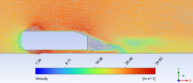
(c) Velocity vector plot

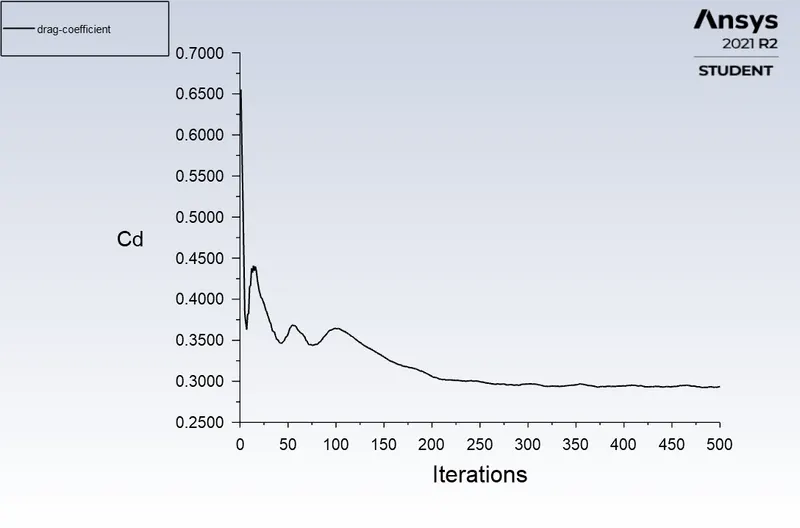
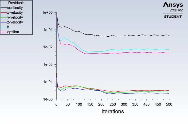
(d) Convergence plots

Figure (5): Refined simulation results

# Conclusion:

The flow features around Ahmed body are captured reasonably well and are similar to available literature [1] and [2].

Hence the meshing method and turbulence modeling used can be employed for studying the flow over Ahmed body with zero yawing angle.

References:

[1]Experiments and numerical simulations on the aerodynamics of the Ahmed body

[2]Flow and Turbulence Structures in the Wake of a Simplified Car Model