Simulation of a 1D Super-sonic nozzle flow simulation using Macormack Method
1D Quasi Supersonic-subsonic nozzle:
Consider isentropic flow through a supersonic-subsonic nozzle as shown in fig(1). Flow at nozzle inlet comes from a reservoir with a very large cross-sectional area (theoretically `A to infty`) and hence inlet velocity is negligible so inlet conditions can be assumed to be stagnant. The flow is locally subsonic at the convergent section, sonic at the throat and supersonic at the divergent section.
Flow properties at the throat are denoted by an asterisk.
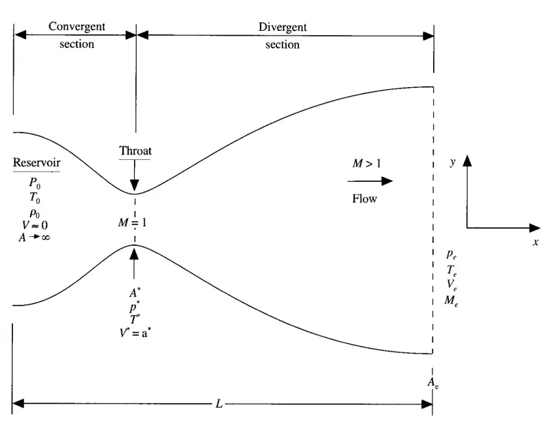
In reality, the flow varies in 2D XY space as the cross-sectional area of the nozzle changes along its length. But we assume that the flow properties are uniform across a given section. Such a flow is called quasi-one-dimensional flow.
Governing Equations :
The non-dimensionalised governing equations are expressed in PDE forms in order to utilise the time marching solution methodology.
Non-conservation form:
Continuity equation :- `(del rho')/(del t') = -rho(del rho')/(del x') -rho'V'(del (ln A'))/(del x') - V'(del rho')/(del x')`
Momentum equation :- `(del V')/(del t') = -V(del V')/(del x') -1/gamma((del T')/(del x') + (T')/(rho')(del rho')/(del x'))`
Energy equation :- `(del T')/(del x') = -V(del T')/(del x') - (gamma-1)T'[(del T')/(del x')+V'(del ln A')/(del x')]`
Conservation form:
Continuity equation :- `(del (rho' A'))/(delt') + (del (rho' A'V'))/(delt') =0`
Momentum equation :- `(del (rho' A'V'))/(del t') + (del [rho' A'V'^2 + (1//gamma)p'A'])/(del x') = 1/gammap'(del A')/(del x')`
Energy equation :- `(del [rho'((e')/(gamma-1) + gamma/2V'^2)A'])/(del t') + (del [rho'((e')/(gamma-1) + gamma/2V'^2)V'A' + rho'A'V'])/(del x') = 0`
where nondimensional variables are,
`T'=T/T_0, rho'=rho/rho_0, V'=V/a_0 " " (a_0=sqrt(gammaRT_0)" is sonic speed at reservoir")`
`A'=A/A^ast, x'=x/L" & "t'=t/(L//a_0)`
To assist the use of MacCormack's technique on equations in conservation form we can make substitutions as:
`U_1=rho'A'`
`U_2=rho'A'V'`
`U_1=rho'((e')/(gamma-1)+ gamma/2V^('2))A'`
`F_1=rho'A'V'`
`F_2=rho'A'V^('2) + 1/gamma p'A'`
`F_3= rho'((e')/(gamma-1)+ gamma/2V^('2))V'A' +rho'A'V^('2)`
`J_2 = 1/gamma p'(delA')/(delx')`
Thus governing equations in conservation form are:
`(del U_1)/(del t') = - (del F_1)/(del x')`
`(del U_2)/(del t') = - (del F_2)/(del x') + J_2`
`(del U_3)/(del t') = - (del F_3)/(del x')`
During time marching will solve for `U_1,U_2" & " U_3` (solution terms) at time step k and then compute `F_1,F_2 " & " F_3`(Flux terms) directly from solution terms so as to reduce rounding errors introduced when finding flux terms from primitive variables. So flux terms (& also source term `J_2`) will be computed as follows:
`F_1 = U_2`
`F_2 = U_2^2/U_1^2 + (gamma-1)/gamma(U_3 - gamma/2U_2^2/U_1^2)`
`F_3 = gamma(U_2U_3)/U_1 - (gamma(gamma-1))/2U_2^3/U_1^2`
`J_2 = (gamma-1)/gamma(U_3 - gamma/2U_2^2/U_1)(del A')/(del x')1/A`
For finding primitive variables at any time step during time marching we can do so using the following equations,
`rho'=U_1/A'` , `V'=U_2/U_1`
`T'=(gamma-1)(U_3/U_1 - gamma/2V^('2))` , `p'=rho'T'`
MacCormack's Technique :
MacCormack method is an explicit finite difference technique that is second-order accurate both in space and time.
The main advantage of this method is that we don't need to compute the second-order time derivative of the function we are solving for but still being able to obtain a 2nd order accurate approximation for the next time step.
For instance consider a function whoose value at next time step is computed as,
`f_i^(t+Deltat) = f_i^t + ((del f)/(del t))_i *Deltat`
1) Predictor step:
In predictor step we use forward differencing for space (not present here) and time derivative as,
`((del f)/(del t))_i^t = (f^t(i+1)-f^t(i))/(Delta t)" "(O Delta x)`
now we use `(del f)/(del t)` to find predicted (because it is only 1st order accurate) value of `f` at next time step,
`barf_i^(t+Delta t) = f_i^t + ((del f)/(del t) )_i^t *Delta t`
2) Corrector step:
In corrector step we use backward differencing & `barf_i^(t+Deltat)` to find predicted value of `(del f)/(del t))` at next time step,
`(bar(del f)/(del t))_i^(t+ Delta t) = (barf^(t + Delta t)(i) - barf^(t + Delta t)(i-1))/(Deltat)`
3) Final time derivative:
So a 2nd order accurate time derivative is the average of above two derivatives computed as,
`((del f)/(del t))_(av) = 1/2(((del f)/(del t))_i^(t) + (bar(del f)/(del t))_i^(t+Delta t))`
`therefore f_i^(t + Delta t) = f_i^t + ((del f)/(del t))_(av)*Delta t`
MATLAB Code for simulating 1D Super-sonic nozzle flow using Macormack Method:
(A) Function code (Non-conservative form)
- The function takes input arguments no. of grid points(n), no. of time steps (nt), Courant no. (C), adiabatic index (`gamma`) and tolerance at convergence (tol).
- Next space grid and area profile are generated followed by initial conditions of non-dimensional variables T,' rho' & v. Also the throat index is calculated.
- Now 3D arrays for variables of interest are initialized with zeros(). Using a 3D array it will be possible to access the value of a variable at any grid point & any time step.
- In the time loop first, the time step size is calculated by applying the CFL condition at all nodes and the min value is assigned to dt.
- Next, values of variables at `k^(th)` time step are stored before the predictor step.
- In the predictor loop, forward differences are applied for space & time derivatives and the predicted values of time derivatives & primitives are computed. The loop runs from 2 to n-1 because inlet and outlet boundary conditions are yet to be set.
- The corrector loop runs in the same way as the predictor loop but without any update of primitive values. The predicted values of time derivatives are stored.
- Now average time derivative is computed followed by primitive variables. At last, the boundary conditions are added and final values are stored in 3D arrays along with info of time step k. Steps 4 to 8 are repeated inside the time loop and the solution time marches with each iteration.
- At the end of the time loop an if condition checks for convergence, returns the last time step (kn) and breaks the time loop thereby ending the function.
-------------------------------------------------------------------------------------------------------------------------------------------
function [rho_t,v_t,T_t,p_t,M_t,mflow_t,kn] = non_conservation_form(n,nt,C,gamma,tol)
x = linspace(0,3,n);              % Space Grid
dx  = x(2) - x(1);                % Space-step
A   = 1 + 2.2*(x - 1.5).^2;       % Area profile (Non-Dimensional)
% getting throat index
if (mod(n,2)==0),throat = n/2; % n is even
else ,throat = (n+1)/2;        % n is odd
end

% Initial Conditions
rho = 1 - 0.3146*x;               % Density (Non-Dimensional)
T   = 1 - 0.2314*x;               % Temperature (Non-Dimensional)
v   = (0.1 + 1.09*x).*(T.^(0.5)); % Velocity (Non-Dimensional)

% Pre-allocating arrays for speed
[drhodt,dvdt,dTdt,drhodt_p,dvdt_p,dTdt_p] = deal(zeros(1,n-1));
[rho_t(:,:,1),v_t(:,:,1),T_t(:,:,1),...
    p_t(:,:,1),M_t(:,:,1),mflow_t(:,:,1)] = deal(zeros(1,n));

% Non-Conservation form of Governing Equ.
    for k = 1:nt
        dt  = min((C*dx)./((T.^0.5)+v));  % Selecting min value of dt
                                          % across all grid points
        % Updating old values
        rho_old = rho;
        T_old = T;
        v_old = v;

        % Predictor Step
        for i = 2:n-1
            % Forward differences (at ith grid point)
            dvdx    = (v(i+1) - v(i))/dx;
            dlogAdx = (log(A(i+1)) - log(A(i)))/dx;
            drhodx  = (rho(i+1) - rho(i))/dx;
            dTdx    = (T(i+1) - T(i))/dx;

            % Time derivatives at (k)th time level
            % Continuity Equation
            drhodt(i) = -rho(i)*dvdx - rho(i)*v(i)*dlogAdx - v(i)*drhodx;
            % Momentum Equation
            dvdt(i)   = -v(i)*dvdx - (1/gamma)*(dTdx + (T(i)/rho(i))*drhodx);
            % Energy Equation
            dTdt(i)   = -v(i)*dTdx - (gamma-1)*T(i)*(dvdx + v(i)*dlogAdx);

            % Solution Update (Predicted values at (k+1)th time level)
            rho(i)  = rho_old(i) + drhodt(i)*dt;
            v(i)    = v_old(i) + dvdt(i)*dt;
            T(i)    = T_old(i) + dTdt(i)*dt;
        end

        % Corrector Step
        for j = 2:n-1
            % Backward differences (at jth grid point)
            dvdx    = (v(j) - v(j-1))/dx;
            dlogAdx = (log(A(j)) - log(A(j-1)))/dx;
            drhodx  = (rho(j) - rho(j-1))/dx;
            dTdx    = (T(j) - T(j-1))/dx;

            % Predicted time derivatives at (k+1)th time level
            % Continuity Equation
            drhodt_p(j) = -rho(j)*dvdx - rho(j)*v(j)*dlogAdx - v(j)*drhodx;
            % Momentum Equation
            dvdt_p(j)   = -v(j)*dvdx - (1/gamma)*(dTdx + (T(j)/rho(j))*drhodx);
            % Energy Equation
            dTdt_p(j)   = -v(j)*dTdx - (gamma-1)*T(j)*(dvdx + v(j)*dlogAdx);
        end

        % Average Time derivatives
        drhodt_av = 0.5*(drhodt + drhodt_p);
        dvdt_av   = 0.5*(dvdt + dvdt_p);
        dTdt_av   = 0.5*(dTdt + dTdt_p);

        % Final Values at time step k+1
        for m = 2:n-1
            rho(m) = rho_old(m) + drhodt_av(m)*dt;
            v(m)   = v_old(m) + dvdt_av(m)*dt;
            T(m)   = T_old(m) + dTdt_av(m)*dt;
        end

        % Boundary Conditions
        % Inlet boundary condition
        v(1)   = 2*v(2) - v(3);
        rho(1) = 1;
        T(1)   = 1;
        % Outlet boundary condition
        v(n)   = 2*v(n-1) - v(n-2);
        rho(n) = 2*rho(n-1) - rho(n-2);
        T(n)   = 2*T(n-1) - T(n-2);

        % Storing timewise variation of variables
        rho_t(:,:,k)   = rho;
        v_t(:,:,k)     = v;
        T_t(:,:,k)     = T;
        p_t(:,:,k)     = rho.*T;
        M_t(:,:,k)     = v./(T.^(0.5));
        mflow_t(:,:,k) = rho.*A.*v;

        % Checking for convergence
        if (k~=1)
           kn = k;              % Returning last timestep value
           error = max(abs(mflow_t(1,throat,k) - mflow_t(1,throat,k-1)));
           if (error < tol)
           break
           end
        end

    end
end
-------------------------------------------------------------------------------------------------------------------------------------------
(B) Function code (Conservative form)
- The function takes input arguments no. of grid points(n), no. of time steps (nt), Courant no. (C), adiabatic index (`gamma`) and tolerance at convergence (tol).
- Next space grid and area profile are generated followed by 3D arrays for variables of interest are initialized with zeros(). Using a 3D array it will be possible to access the value of a variable at any grid point & any time step. Also, the throat index is calculated.
- Now nondimensional variables T,' rho',v', u1, u2 & u3 are generated with initial conditions.
- In the time loop first, the time step size is calculated by applying the CFL condition at all nodes and the min value is assigned to dt.
- Next, values of solution variables at `k^(th)` time step are stored before the predictor step while flux variables are re-calculated.
- In the predictor loop, forward differences are applied for space & time derivatives and the predicted values of time derivatives, solution variables & flux variables are computed. The loop runs from 2 to n-1 because inlet and outlet boundary conditions are yet to be set.
- The corrector loop runs in the same way as the predictor loop but without any update of solution or flux variables. The predicted values of time derivatives are stored.
- Now average time derivative is computed followed by primitive variables. At last, the boundary conditions are added and final computed values of primitive variables are stored in corresponding 3D arrays along with info of time step k. Steps 4 to 8 are repeated inside the time loop and the solution time marches with each iteration.
- At the end of the time loop an if condition checks for convergence, returns the last time step (kn) and breaks the time loop thereby ending the function.
-------------------------------------------------------------------------------------------------------------------------------------------
function [rho_t,v_t,T_t,p_t,M_t,mflow_t,kn] = conservation_form(n,nt,C,g,tol)

x = linspace(0,3,n);              % Space Grid
dx  = x(2) - x(1);                % Space-step
A   = 1 + 2.2*(x - 1.5).^2;       % Area profile (Non-Dimensional)
% getting throat index
if (mod(n,2)==0),throat = n/2; % n is even
else ,throat = (n+1)/2;        % n is odd
end

% Preallocating arrays for speed
[du1dt,du2dt,du3dt,du1dt_p,du2dt_p,du3dt_p] = deal(zeros(1,n-1));
[rho_t(:,:,1),v_t(:,:,1),T_t(:,:,1),...
      p_t(:,:,1),M_t(:,:,1),mflow_t(:,:,1)] = deal(zeros(1,n));
                                    [rho,T] = deal(zeros(1,n));

% Initial Conditions
for z = 1:n
    if x(z)<=0.5
        rho(z) = 1;               % Density (Non-Dimensional)
        T(z)   = 1;               % Temprature (Non-Dimensional)
    elseif (x(z)>0.5) && (x(z)<=1.5)
        rho(z) = 1-0.366*(x(z) - 0.5);
        T(z)   = 1 - 0.167*(x(z) - 0.5);
    elseif (x(z)>1.5) && (x(z)<=3.5)
        rho(z) = 0.634 - 0.3879*(x(z) - 1.5);
        T(z)   = 0.833 + 0.3507*(x(z) - 1.5);
    end
end
v   = (0.59)./(rho.*A); % Velocity (Non-Dimensional)
u1  = rho.*A;
u2  = 0.59*ones(1,n);
u3  = u1.*((T/(g-1)) + (g/2).*(v.^2));

% Conservation form of Governing Equ.
   for k = 1:nt
        dt  = min((C*dx)./((T.^0.5)+v));  % Selecting min value of dt
                                          % across all grid points
        % Updating old values
        u1_old  = u1;
        u2_old  = u2;
        u3_old  = u3;
        % Flux terms at kth time level
        f1 = u2;
        f2 = ((u2.^2)./u1) +((g-1)/g)*(u3 - (g/2)*(u2.^2)./u1);
        f3 = ((g*u2.*u3)./u1) - ((g*(g-1)/2)*(u2.^3)./(u1.^2));

        % Predictor Step
        for i = 2:n-1
            % Foreward differences (at ith grid point)
            % Source term
            dAdx = (A(i+1)-A(i))/dx;
            j2   = ((g-1)/g)*(u3(i) - 0.5*g*((u2(i)^2)/u1(i)) )*dAdx/A(i);

            % Continuity equation
            du1dt(i) = -(f1(i+1) - f1(i))/dx;
            % Momentum equation
            du2dt(i) = -(f2(i+1) - f2(i))/dx + j2;
            % Energy equation
            du3dt(i) = -(f3(i+1) - f3(i))/dx;

            % Solution update (predicted values)
            u1(i) = u1_old(i) + du1dt(i)*dt;
            u2(i) = u2_old(i) + du2dt(i)*dt;
            u3(i) = u3_old(i) + du3dt(i)*dt;

            % Predicted values of fluxes
            f1(i) = u2(i);
            f2(i) = ((u2(i)^2)/u1(i)) +((g-1)/g)*(u3(i) - (g/2)*(u2(i)^2)/u1(i));
            f3(i) = ((g*u2(i)*u3(i))/u1(i)) - ((g*(g-1)/2)*(u2(i)^3)/(u1(i)^2));
        end

        % Corrector Step
        for j = 2:n-1
            % Backward differences (at jth grid point)
            % Source term
            dAdx = (A(j)-A(j-1))/dx;
            j2   = ((g-1)/g)*(u3(j) - 0.5*g*((u2(j)^2)/u1(j)))*dAdx/A(j);

            % Continuity equation
            du1dt_p(j) = -(f1(j) - f1(j-1))/dx;
            % Momentum equation
            du2dt_p(j) = -(f2(j) - f2(j-1))/dx + j2;
            % Energy equation
            du3dt_p(j) = -(f3(j) - f3(j-1))/dx;
        end

        % Average Time derivatives
        du1dt_av   = 0.5*(du1dt + du1dt_p); % drhodt_av
        du2dt_av   = 0.5*(du2dt + du2dt_p);
        du3dt_av   = 0.5*(du3dt + du3dt_p);

        % Final Values at (k+1)th time step
        for m = 2:n-1
            u1(m) = u1_old(m) + du1dt_av(m)*dt;
            u2(m) = u2_old(m) + du2dt_av(m)*dt;
            u3(m) = u3_old(m) + du3dt_av(m)*dt;
        end

        % Boundary Conditions
        % Inlet boundary condition
        u1(1)  = A(1);
        u2(1)  = 2*u2(2) - u2(3);
        u3(1)  = u1(1)*( (T(1)/(g-1)) + (g/2)*((u2(1)/u1(1))^2) );
        % Outlet boundary condition
        u1(n)   = 2*u1(n-1) - u1(n-2);
        u2(n)   = 2*u2(n-1) - u2(n-2);
        u3(n)   = 2*u3(n-1) - u3(n-2);

        % Fluid properties at (k+1)th time step
        rho = u1./A;
        v   = u2./u1;
        T   = (g-1)*((u3./u1) - (g/2)*((u2./u1).^2));

        % Storing timewise variation of variables
        rho_t(:,:,k)   = rho;
        v_t(:,:,k)     = v;
        T_t(:,:,k)     = T;
        p_t(:,:,k)     = rho.*T;
        M_t(:,:,k)     = v./(T.^(0.5));
        mflow_t(:,:,k) = rho.*A.*v;


        % Checking for convergence
        if (k~=1)
           kn = k;              % Returning last timestep value
           error = max(abs(mflow_t(1,throat,k) - mflow_t(1,throat,k-1)));
           if (error < tol)
           break
           end
        end

    end
end
------------------------------------------------------------------------------------------------------------------------------------
(C) Main code:
- First Inputs to the functions above are defined and then the functions are called. Their outputs are stored in different variables.
- In code block, 1 3D array indices (1,:,kn) are used to access the values computed at the last time step when the convergence condition was met.
- In block 2 time-wise variation of mass flow rate is plotted using only the index as (:,:,k). Now code blocks 1 & 2 are looped 2 times calling different functions.
- In block 3 we use the squeeze() function so that the 3D array reduces to a 1xkn array at throat index which matches dimensions 1xkn of the x-axis in the plot.
- In block 4 we use the same array indexing as in block 1 i.e. (1,:,kn). The outputs from both functions are plotted with the analytical solution. The mean mass flow rate across all grid points is computed for both functions and results are tabulated for comparison against mass flow rate using an analytical solution.
- In block 5, we perform a grid independence test. Inside a for loop functions are called with different no. of grid points and density, temperature,mach no. & pressure profile is obtained from both functions. The values are stored in the respective 3x1 array variables. The results are then tabulated.
-------------------------------------------------------------------------------------------------------------------------------------------
clearvars
close all
clc
% Inputs
n     = 31;        % No. of grid points
nt    = 1400;       % No. of time steps
gamma = 1.4;        % Heat capacity ratio
C     = 0.5;        % Courant Number
tol   = 1e-8;       % Error tolerance at convergence

% Solving
[rho1,v1,T1,p1,M1,mflow_nc,kn1] = non_conservation_form(n,nt,C,gamma,tol);
[rho2,v2,T2,p2,M2,mflow_c,kn2] = conservation_form(n,nt,C,gamma,tol);

x = linspace(0,3,n);
str1 = ["(Non-Conservation form)" "(Conservation form)"];

for j = 1:2
 % Distributing variables
 if  j==1 , [rho,v,T,p,M,mflow,kn] = deal(rho1,v1,T1,p1,M1,mflow_nc,kn1);
 else ,    [rho,v,T,p,M,mflow,kn] = deal(rho2,v2,T2,p2,M2,mflow_c,kn2);end

% BLOCK 1: Plotting Steady state distribution of variables inside nozzle
figure('position',[300 100 1000 400])
plot(x,v(1,:,kn),'b',x,T(1,:,kn),'r',x,rho(1,:,kn),'g',x,p(1,:,kn),'m')
legend({'Velocity','Density','Temperature','Pressure'},'location','northwest')
xlabel('Nozzle length ( x / L ) rightarrow')
ylabel('Non-dimensional variables rightarrow')
title('Steady state distribution of primitive variables')
subtitle(str1(j))


% BLOCK 2: Plotting timewise variation of massflow rate along nozzle length
figure('position',[300 100 1000 500])
clr = ["-.b" "c" "y" "g" "m" "xr" "k"];
i   = 1;
for k = 1:nt
    if ismember(k,[1 50 100 150 200 700 kn])
    plot(x,mflow(:,:,k),clr(i),'linewidth',0.9)
    hold on
    i = i+1;
    end
end
str2 = ["1Deltat","50Deltat","100Deltat",...
    "150Deltat","200Deltat","700Deltat",kn + "Deltat"];
legend(str2,'location','north','NumColumns',2)
xlabel('Nozzle length ( x / L ) rightarrow')
ylabel('Mass flow rate  ( rho / rho* ) rightarrow')
title('Transient variation of Mass flow rate (Non-dimensional)')
subtitle(str1(j));
hold off

end

% BLOCK 3: Plotting timewise variaton of variables at throat
% getting throat index
if (mod(n,2)==0),throat = n/2; % n is even
else ,throat = (n+1)/2;        % n is odd
end
figure('position',[300 100 1000 500])
t = tiledlayout(4,1);

nexttile
plot(1:kn1, squeeze(v1(1,throat,:)) ,'g','linewidth',0.8);
hold on
plot(1:kn2, squeeze(v2(1,throat,:)) ,'k','linewidth',0.8);
title('Velocity')
legend('Non-conservation form','Conservation form')

nexttile
plot(1:kn1, squeeze(p1(1,throat,:)) ,'r','linewidth',0.8);
hold on
plot(1:kn2, squeeze(p2(1,throat,:)) ,'k','linewidth',0.8);
title('Pressure')
legend('Non-conservation form','Conservation form')

nexttile
plot(1:kn1, squeeze(T1(1,throat,:)) ,'b','linewidth',0.8);
hold on
plot(1:kn2, squeeze(T2(1,throat,:)) ,'k','linewidth',0.8);
title('Temperature')
legend('Non-conservation form','Conservation form')

nexttile
plot(1:kn1, squeeze(rho1(1,throat,:)) ,'m','linewidth',0.8);
hold on
plot(1:kn2, squeeze(rho2(1,throat,:)) ,'k','linewidth',0.8);
title('Density')
legend('Non-conservation form','Conservation form')

xlabel(t,'Time steps rightarrow')
ylabel(t,'Non-dimensional variable rightarrow')
title(t,'Transient variation of Non-dimensional variables')
subtitle(t,'(At nozzle throat)')

%BLOCK 4: Comparison of Normalized mass flow rate distributions of both forms
figure('position',[300 100 1000 500])
plot(x,mflow_nc(1,:,kn1),'m','linewidth',1)
hold on
plot(x,mflow_c(1,:,kn2),'b','linewidth',1)
plot(x,0.579*ones(1,n),'g','linewidth',1)
legend({'Non-Consevation Form','Consevation Form','Analytical Solution'},'location','north')
title('Comparison of Normalized mass flow rate distributions of both forms')
subtitle('(Steady state)')
xlabel('Nozzle length ( x / L ) rightarrow')
ylabel('Mass flow rate  ( rho / rho* ) rightarrow')

row_tab1 = ["Non-conservation form";"Conservation form"];
Steady_state_mean_mfr  = [mean(mflow_nc(1,:,kn1));mean(mflow_c(1,:,kn2))];
Analytical_mfr         = [0.579;0.579];
Error_percent          = 100*(Steady_state_mean_mfr - Analytical_mfr);
Iterations_to_converge = [kn1;kn2];
tab1 = table(Steady_state_mean_mfr,Analytical_mfr,Error_percent,...
                Iterations_to_converge,'rownames',row_tab1);
disp(tab1)

% BLOCK 5: Grid Independence test
gp = [31,62,93];
for j = 1:3
% [rho_t,v_t,T_t,p_t,M_t,mflow_t,kn]
[rho1,v1,T1,p1,M1,mfr1,kn1]= non_conservation_form(gp(j),nt,C,gamma,tol);
[rho2,v2,T2,p2,M2,mfr2,kn2]  = conservation_form(gp(j),nt,C,gamma,tol);
% getting throat index
if (mod(gp(j),2)==0),throat = gp(j)/2; % n is even
else ,throat = (gp(j)+1)/2; end        % n is odd

Density_NC(j,1)     = rho1(1,throat,kn1);
Temperature_NC(j,1) = T1(1,throat,kn1);
Pressure_NC(j,1)    = p1(1,throat,kn1);
Mach_no_NC(j,1)     = M1(1,throat,kn1);

Density_C(j,1)     = rho2(1,throat,kn2);
Temperature_C(j,1) = T2(1,throat,kn2);
Pressure_C(j,1)    = p2(1,throat,kn2);
Mach_no_C(j,1)     = M2(1,throat,kn2);
end

fprintf('n                              [GRID INDEPENDENCE TEST]')
fprintf('nFor Non-conservation form:n')
Grid_Points = num2str(gp');
tab2 = table(Grid_Points,Density_NC,Temperature_NC,Pressure_NC,Mach_no_NC);
disp(tab2)
fprintf('For Conservation form:n')
tab3 = table(Grid_Points,Density_C,Temperature_C,Pressure_C,Mach_no_C);
disp(tab3)
% END OF PROGRAM
-------------------------------------------------------------------------------------------------------------------------------------------
PROGRAM OUTPUTS & INFERENCES:
(1) Variation of flow properties at throat:-
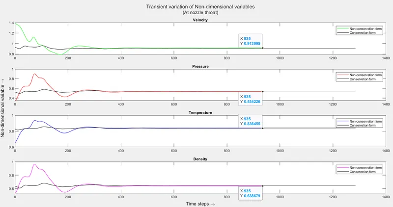
- From the above plot, we can see that the conservation form handles shocks in the physical system much better than the non-conservative form. This is due to the fact that the conservation form uses solution variables which are fluxes of mass, momentum and internal energy. The flux variables are constant across a shock and are changed only due to numerical errors.
(2) Variation in mass flow rate:-
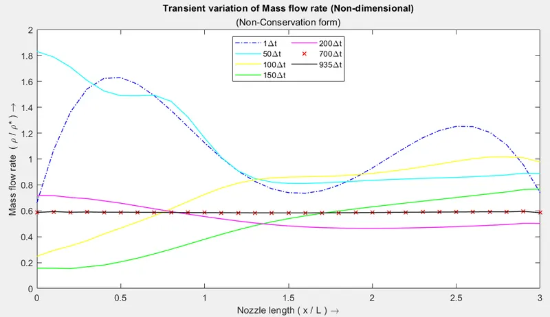
- The mass flow rate plot shows the initial profile with blue.
- The profile is changing rapidly with huge variations until 200 th time step after which it becomes closer to the steady-state profile.
- The profile converges after 935 iterations with an error tolerance of `10^(-8)` for mass flow rate.
- The solution converges close to 0.579 the exact analytical value.
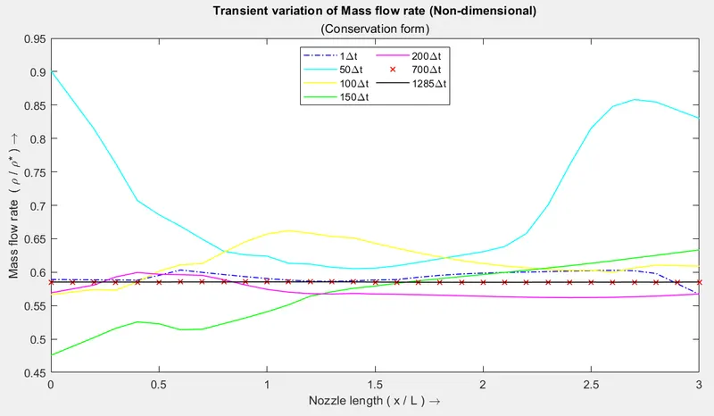
- The mass flow rate plot shows the initial profile with blue.
- Again we see huge variations until the 200 th time step after which the profile stabilises.
- The profile converges after 1285 iterations in a time loop with an error tolerance of `10^(-8)` for mass flow rate.
- It converges slower than the non-conservation form because converting flux solution variables back to primitive variables introduce rounding off errors.
- The profile converges close to 0.579 the exact analytical value.
(3) Comparison of normalized mass flow rate profiles:
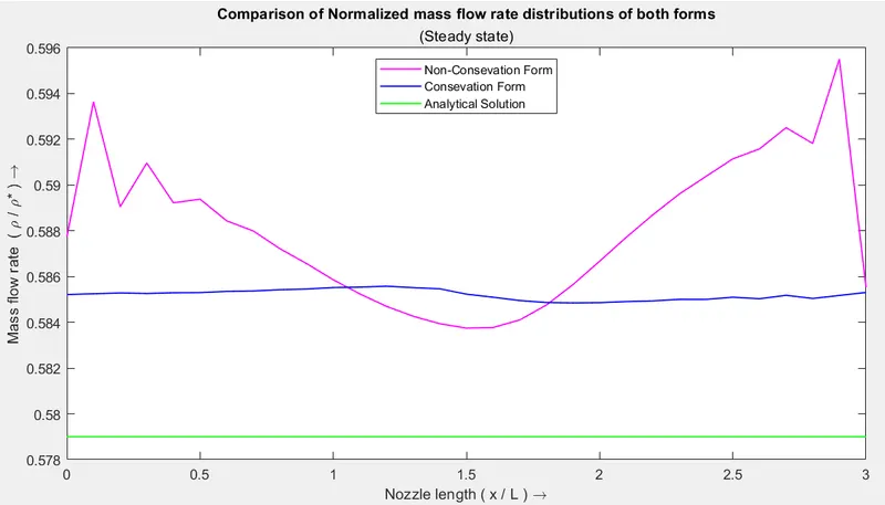
- Both the forms of governing equations are undoubtedly stable. But conservative form computes mass flow rate more accurate than the non-conservation form.
- This is due to the fact that the conservation form uses flux variables that are conserved throughout the flow field.
- But non-conservation form converges faster because it directly solves the primitive variables while the conservation form is subjected to rounding off errors during the calculation of primitives from flux solution variables.
(4) Steady-state distribution of primitive variables:
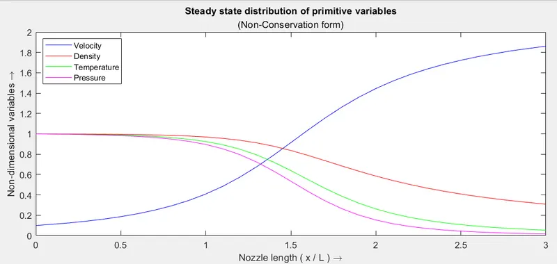
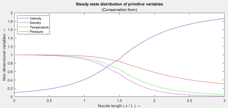
- The steady-state primitive variables obtained from both forms of governing equations are satisfactory.
- The velocity is increasing along with the nozzle as expected. However, density, temperature and pressure are dropping continuously with increasing velocity.
(5) Grid Independence Test:
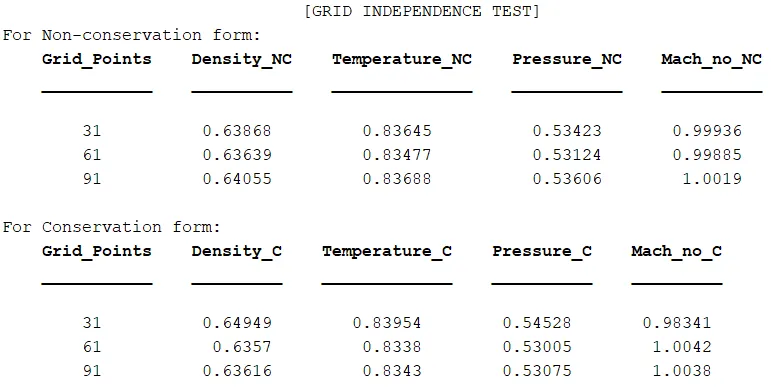
- We know that as the grid becomes finer increase numerical errors decrease and the solution becomes more accurate. This is why we need to make sure that our solution is accurate to desired decimal points and is independent of the grid.
- From the above plots, we can see that even on doubling & tripling grid points the results have minor changes but are practically the same.
- So the solution can be called grid independent for 31 grid points.
- Again we can see that the non-conservation form finds primitive variables more accurately than the conservation form.