Deriving 4th order approximation of a 2nd order derivative using Taylor Table method

Central difference scheme :

In this scheme derivative at a point is approximated by taking information about two points ahead and two points behind the point under consideration. For symmetric `4^(th)` order approximation of a second-order derivative,

`"Number of nodes in stencil " = " Order of accuracy"+"Order of derivative"-1 = 4+2-1=5`

So our numerical stencil is,

Let the hypotheisis function be,

`Delta x^2(d^2u)/(dx^2)= af(i-2)+bf(i-1)+cf(i)+df(i+1)+ef(i+2)......(1)`

by using Taylor series expansion (upto 7 terms) the above equation can be written as,

`Delta x^2(d^2u)/(dx^2) = Kf(i)+ADelta xf'(i)+BDelta x^2f''(i)+CDelta x^3f'''(i)+DDelta x^4f^((4))(i)+EDelta x^5f^((5))(i)+GDelta x^6f^((6))(i)......(2)`

where K, A, B, C, D, E & G are constant coefficients in respective terms.

Now using Taylor table method,

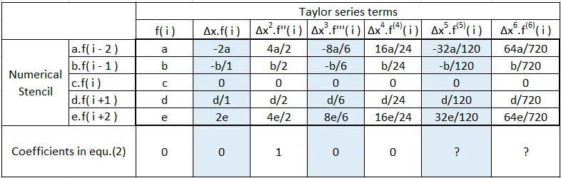
so we get following equations,

`a+b+c+d+e=0`

`-2a-b+0+d+2e=0`

`(4a)/2+b+0+d/2+(4e)/2=1`

`-(8a)/6-b/6+0+d/6+(8e)/6=0`

`(16a)/24+b/24+0+d/24+(16e)/24=0`

Since we want to approximate the `d^2u//dx^2` coefficient of `Delta x^2.f''(i)` must be equal to `1` and for other terms, the coefficients should be `0` except for `Delta x^5.f^((5))(i)" & "Delta x^6.f^((6))(i)`. This because we have `5` unknowns that need `5` equations to give us a unique solution so specifying the coefficient of terms beyond `Delta x^4f^((4))(i)` will over constraint the solution which may lead to inappropriate results.

Solving the above set of equations in MATLAB,

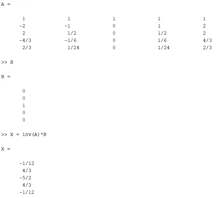
We get,

`a=e=-1/12,c=-5/2" & " b=d=4/3`

from equ.`(2)`,

`Delta x^2(d^2u)/(dx^2) = BDelta x^2f''(i)+EDelta x^5f^((5))(i)+GDelta x^6f^((6))(i)`

`therefore Delta x^2(d^2u)/(dx^2) = (1)Delta x^2f''(i)+((-32a-b+0+d+32e)/120)Delta x^5f^((5))(i)+GDelta x^6f^((6))(i)`

`therefore Delta x^2(d^2u)/(dx^2) = Delta x^2f''(i)+(0)Delta x^5f^((5))(i)+GDelta x^6f^((6))(i)" "(because a=e and b=d)`

We find that coefficient of `Delta x^5f^((5))(i)` is also zero but not of `Delta x^6f^((6))(i)` and on dividing by `Delta x^2` on both sides the highest power of `Delta x` is 4. This term will be truncated so our approximation in `4^(th)` order accurate,

`(d^2u)/(dx^2) = f''(i)+GDelta x^4f^((6))(i)=(af(i-2)+bf(i-1)+cf(i)+df(i+1)+ef(i+2))/(Delta x^2)+ O(Delta x)^4`

`therefore (d^2u)/(dx^2) = ( -1/12f(i-2)+4/3f(i-1)-5/2f(i)+4/3f(i+1)-1/12f(i+2))/(Delta x^2)`

simplyfying,

`therefore (d^2u)/(dx^2) = (-f(i-2)+16f(i-1)-30f(i)+16f(i+1)-f(i+2))/(12Delta x^2)`

Skewed right-sided difference:

In this scheme derivative at a point is approximated by taking information from five points ahead the point under consideration. For symmetric `4^(th)` order approximation of a second-order derivative,

`"Number of nodes in stencil " = " Order of accuracy"+"Order of derivative" = 4+2=6`

So our numerical stencil is,

Let the hypotheisis function be,

`Delta x^2(d^2u)/(dx^2)= af(i)+bf(i+1)+cf(i+2)+df(i+3)+ef(i+4)+gf(i+5)......(5)`

by using Taylor series expansion (upto 7 terms) the above equation can be written as,

`Delta x^2(d^2u)/(dx^2) = Kf(i)+ADelta xf'(i)+BDelta x^2f''(i)+CDelta x^3f'''(i)+DDelta x^4f^((4))(i)+EDelta x^5f^((5))(i)+GDelta x^6f^((6))(i)......(6)`

where K, A, B, C, D, E & G are constant coefficients in respective terms.

Now using the Taylor table method,

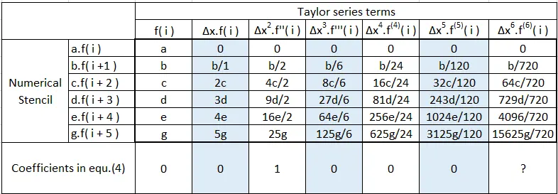
Since we want to approximate the `d^2u//dx^2` coefficient of `Delta x^2.f''(i)` must be equal to `1` and for other terms, the coefficients should be `0` except for `Delta x^6.f^((6))(i)`. This because we have `6` unknowns that need `6` equations to give us a unique solution so specifying the coefficient of terms beyond `Delta x^5f^((4))(i)` will over constraint the solution which may lead to inappropriate results.

Solving the coefficient equations in MATLAB,

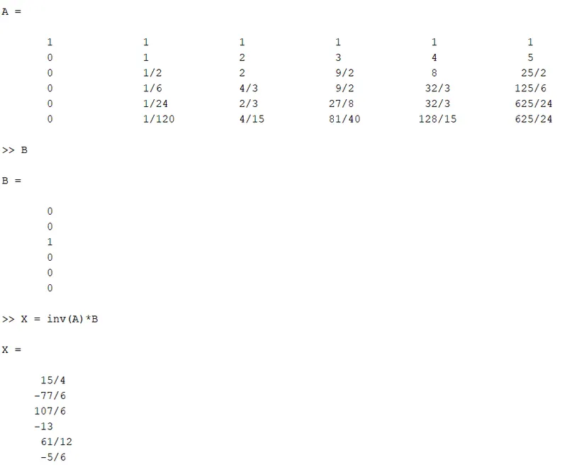
We get,

` a=15/4, b=-77/6, c=107/6, d=-13, e=61/12" & "g=-5/6`

from equ.`(4)`,

`Delta x^2(d^2u)/(dx^2) = (1)Delta x^2f''(i)+GDelta x^6f^((6))(i)`

on dividing by `Delta x^2` on both sides the highest power of `Delta x` is 4. This term will be truncated so our approximation in `4^(th)` order accurate,

`(d^2u)/(dx^2) = f''(i)+O(Delta x)^4`

`(d^2u)/(dx^2) = (af(i)+bf(i+1)+cf(i+2)+df(i+3)+ef(i+4)+gf(i+5))/(Delta x^2)`

`therefore (d^2u)/(dx^2) = (15/4f(i)-77/6f(i+1)+107/6f(i+2)-13f(i+3)+61/12f(i+4)-5/6f(i+5))/(Delta x^2)`

Simplyfying,

`therefore (d^2u)/(dx^2) = (45f(i)-154f(i+1)+214f(i+2)-156f(i+3)+61f(i+4)-10f(i+5))/(12Delta x^2)`

Skewed left-sided difference:

In this scheme derivative at a point is approximated by taking information from five points behind the point under consideration. For symmetric `4^(th)` order approximation of a second-order derivative,

`"Number of nodes in stencil " = " Order of accuracy"+"Order of derivative" = 4+2=6`

So our numerical stencil is,

Let the hypotheisis function be,

`Delta x^2(d^2u)/(dx^2)= af(i)+bf(i-1)+cf(i-2)+df(i-3)+ef(i-4)+gf(i-5)......(3)`

by using Taylor series expansion (upto 7 terms) the above equation can be written as,

`Delta x^2(d^2u)/(dx^2) = Kf(i)+ADelta xf'(i)+BDelta x^2f''(i)+CDelta x^3f'''(i)+DDelta x^4f^((4))(i)+EDelta x^5f^((5))(i)+GDelta x^6f^((6))(i)......(4)`

where K, A, B, C, D, E & G are constant coefficients in respective terms.

Now using the Taylor table method,

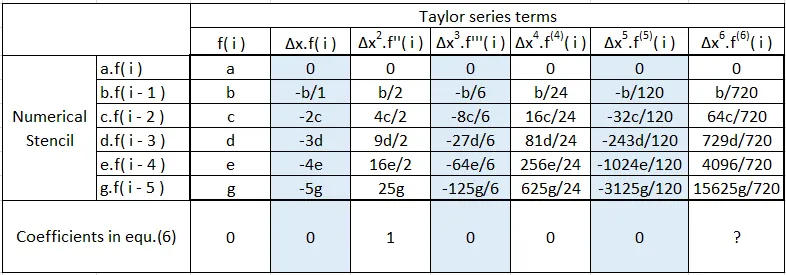
Since we want to approximate the `d^2u//dx^2` coefficient of `Delta x^2.f''(i)` must be equal to `1` and for other terms, the coefficients should be `0` except for `Delta x^6.f^((6))(i)`. This because we have `6` unknowns that need `6` equations to give us a unique solution so specifying the coefficient of terms beyond `Delta x^5f^((4))(i)` will over constraint the solution which may lead to inappropriate results.

Solving the coefficient equations in MATLAB,

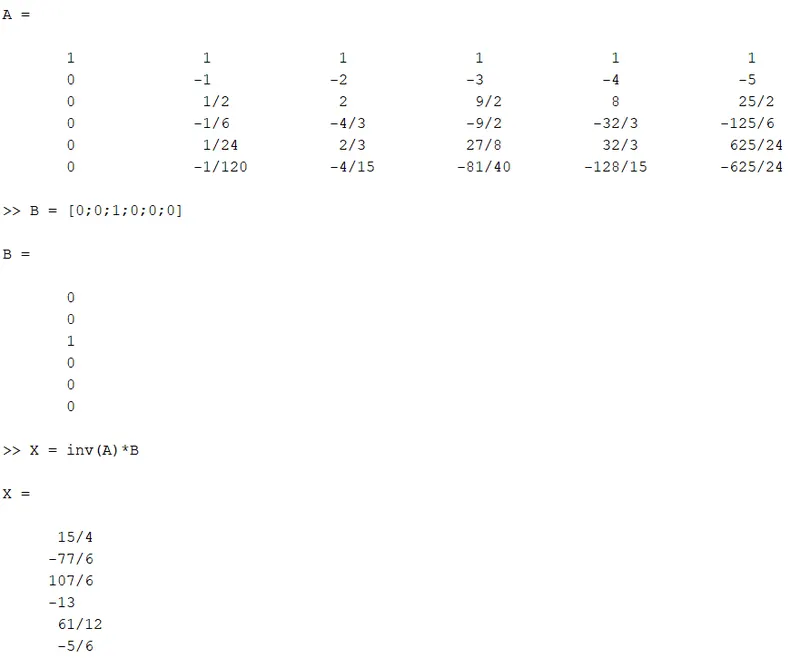
We get,

` a=15/4, b=-77/6, c=107/6, d=-13, e=61/12" & "g=-5/6`

from equ.`(6)`,

`Delta x^2(d^2u)/(dx^2) = (1)Delta x^2f''(i)+GDelta x^6f^((6))(i)`

on dividing by `Delta x^2` on both sides the highest power of `Delta x` is 4. This term will be truncated so our approximation in `4^(th)` order accurate,

`(d^2u)/(dx^2) = f''(i)+O(Delta x)^4`

`(d^2u)/(dx^2) = (af(i)+bf(i-1)+cf(i-2)+df(i-3)+ef(i-4)+gf(i-5))/(Delta x^2)`

`therefore (d^2u)/(dx^2) = (15/4f(i)-77/6f(i-1)+107/6f(i-2)-13f(i-3)+61/12f(i-4)-5/6f(i-5))/(Delta x^2)`

Simplyfying,

`therefore (d^2u)/(dx^2) = (45f(i)-154f(i-1)+214f(i-2)-156f(i-3)+61f(i-4)-10f(i-5))/(12Delta x^2)`

MATLAB Coding for Numerical second derivative:

1. First, we will define the mathematical function `f(x)=e^x cos x` in MATLAB which is,

       function out = f1(x)
           out = exp(x)*cos(x);
       end​

2. The next three functions are defined which take arguments a_der (analytical derivative), x and dx (or `Deltax`); calls function f1, computes fourth-order approximations of `f''(x)` using central difference, skewed right-sided & skewed left-sided schemes respectively and then outputs the absolute difference between analytical and numerical derivative.

   function error = cal_cds_error (a_der,x,dx)
    % Numerical second derivative
     central_diff_scheme = (-f1(x-2*dx)+16*f1(x-dx)-30*f1(x)+16*f1(x+dx)-f1(x+2*dx))/(12*(dx^2));
     error = abs(a_der - central_diff_scheme);
   end​

   function error = cal_srss_error (a_der,x,dx)
     % Numerical second derivative
     skewed_right_sided = (45*f1(x)-154*f1(x+dx)+214*f1(x+2*dx)-156*f1(x+3*dx)+61*f1(x+4*dx)-10*f1(x+5*dx))/(12*(dx^2));
     error = abs(a_der -  skewed_right_sided);
   end

   function error = cal_slss_error (a_der,x,dx)
     % Numerical second derivative
     skewed_left_sided =(45*f1(x)-154*f1(x-dx)+214*f1(x-2*dx)-156*f1(x-3*dx)+61*f1(x-4*dx)-10*f1(x-5*dx))/(12*(dx^2));
     error = abs(a_der - skewed_left_sided);
   end

3. In the main code, we will first calculate the analytical second derivative of `f(x)` i.e. `f''(x)=-2e^x sin x` at `x=pi//3` and then assign the errors in numerical approximation of `f''(x)` for different numerical schemes for varying values of `dx` to three array variables. Lastly, we will plot a graph for comparing the magnitude of errors in different schemes.

   close all
   clear all
   clc
   
   % Analytical function f(x)= exp(x)*cos(x)
   % Analytical second derivative f''(x)= -2*exp(x)*sin(x)
   x = pi/3;
   a_derivative = -2*exp(x)*sin(x);
   
   % Finding absolute error in Numerical Derivative
   dx = linspace(7/10,1/100,30);     % Grid spacing (mesh grid for 3D)
   
   cds_error = zeros(1,30);          % Pre-allocating arrays for faster
   srss_error = zeros(1,30);         % program execution
   slss_error = zeros(1,30);
   
   for i = 1:length(dx)
      cds_error(i)  = cal_cds_error(a_derivative,x,dx(i));
      srss_error(i) = cal_srss_error(a_derivative,x,dx(i));
      slss_error(i) = cal_slss_error(a_derivative,x,dx(i));
   end
   
   % Plotting graph
   loglog(dx,cds_error,'d-','color','b');
   hold on
   loglog(dx,srss_error,'s-','color','k');
   hold on
   loglog(dx,slss_error,'o-','color','r');
   
   xlabel('dx (Grid spacing)');
   ylabel('Absolute error');
   legend('Central difference of 4th order','Skewed right side difference of 4th order','Skewed left side difference of 4th order');
   title('Consistency of different schemes');
   % END OF PROGRAM​

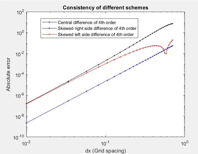
Program output:-

Conclusion:

• The approximation error is least in the central difference scheme as shown from the plot.
• The only limitation of the central difference scheme is that it can't be applied at domain boundaries, due to the lack of left and right nodes simultaneously. So, skewed difference schemes are used at domain boundaries instead.