Validation studies of Symmetry BC vs Wedge BC in OpenFOAM vs Analytical Hagen-Poiseuille equation
# Abstract :
We are going to simulate the internal flow of a fluid through a pipe. The simulation will be validated using the Hagen-Poiseuille equation which is based on the following assumptions:-
- The pipe is horizontal (i.e. no pressure drop due to gravity.
- Fluid sticks at pipe surfaces i.e. no-slip condition at pipe surfaces.
- The fluid is Newtonian & incompressible.
- Flow is laminar, steady & irrotational.
- Flow is 1D i.e fluid velocity varies along radial direction only.
- No acceleration of fluid in pipe i.e. flow occurs at a constant pressure difference.
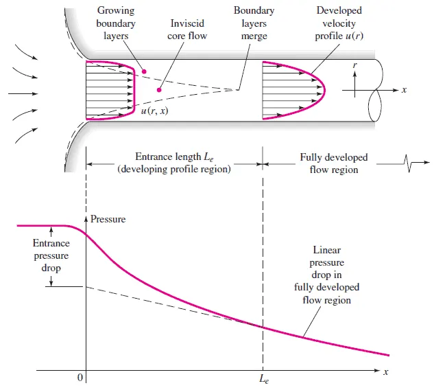
Image source: White Frank M., Fluid Mechanics, McGraw-Hill Education, 7th edition, February,2010, ISBN: 978-0077422417
In real flow, fluid velocity varies along a certain distance from pipe entrance before it becomes invariant with pipe length. This distance is called hydrodynamic entrance length. It is given by,
`L_e/D=0.05Re" (For incompressible laminar flow)"`
The flow should be fully developed for simulating 1D flow, we will account for this by adding entrance length to our simulation model.
# Wedge boundary condition:
- The wedge boundary condition (BC) is used in computational fluid dynamics to define an axisymmetric situation, for eg. cylinder. The model and flow must be axisymmetric along a central line such that all physical variables of the flow have the same value and distribution at a given radius for all angles.
- This boundary condition is specified by two planes that must be selected on separate sides of the domain (referred to as front and back) on surfaces running along the axis.
- It works for 2D simulations only and the flow geometry needs to be specified as a wedge with a small angle (<5 degrees) and a single cell thickness along the curvature.
- Wedge BC applies the Navier-Stokes equations in cylindrical coordinates.
# Symmetry boundary condition:
- The symmetry boundary condition defines a mirror face/surface. It should only be used if the expected flow field pattern of the developed solution are mirrored along that surface.
- By using this boundary condition, the domain can essentially be halved, reducing the time to achieve a solution.
- It can be applied to both planar or non-planar faces/surfaces on the domain boundaries.
- Symmetry BC applies the Navier-Stokes equations in cartesian coordinates.
# Hagen-Poiseuille Equation:
Hagen-Poiseuille Equation finds head loss due to viscosity of fluid for length L (m) along pipe (in fully developed region),
`(P_2−P_1)/(ρg)=h_f=(32μUL)/(ρgD^2)`
Where `mu="dynamic viscosity in Pa-s"`,
`U= "Velocity along pipe length " (m//s)`
`D= "Pipe diametre " (m)`
`ρ= "Density of fluid " (kg//m^3)`
`g= "Acceleraton due to gravity " (m//s^2)`
other equations that are derieved for this Poiseuille flow and valid at any section (in FDF region) are,
Shear stress at radial distance r from pipe centre,
`τ=−(∂P)/(∂x)r/2=−mu(∂U)/(∂r)`
Velocity at radial distance r from pipe centre,
`U=−1/(4μ)(∂P)/(∂x)[R^2−r^2]`
Average velocity across section,
`barU=1/(8μ)(∂P)/(∂x)R^2`
# Calculations :
we will assume the pipe diametre of 2 cm and `R_e=2100`. Also we will assume NTP conditions so,
Density,`" "ρ=998.19" "kg//m^3`
Dynamic viscosity ,`" "mu=1.002"x"10^(−3)" "Ns//m^2`
Kinematic viscosity,`" "nu=1.004"x"10^(−6)" "m^2//s`
initial velocity,`" "U=(R_e nu)//D=0.105" "m//s`
Entrance length,`" "L_e=0.05R_eD=2.1" "m`
Pipe length,`" "L=3" "m (>L_e)`
# Auto generating blockMeshDict file using MATLAB :
For specifying symmetry BC in OpenFOAM, we just need to replace keyword "wedge" with "symmetry" in blockMeshDict, 0/U & 0/p files. So we created two case files HPpipe_W & HPpipe_S with respective keywords.
The MATLAB code below takes pipe diametre, length, wedge angle and type of BC (symmetry or wedge) for generating blockMeshDict file. Based on user inputs the corresponding file is edited.
The code edits three lines in already written file. Changing these lines changes the geometry of our mesh accordingly.
clearvars
close all
clc

% Generating user interface
prompt   = ["Pipe diametre ( m ):-",...
            "Pipe length ( m ):-", ...
            {"Wedge angle for mesh generation ( in Deg"+char(176)+" )"}...
            "Boundary Condition wedge or symmetry (w or s)?"];
dlgtitle =  "Inputs for generating blockMeshDict file";
dims     = [1 70];
definput = ["0.02" "3" "4" "s"];
answer = inputdlg(prompt,dlgtitle,dims,definput);

if isempty(answer)
    msgbox(' Mesh file not updated.','Aborted','error')
    return
end
% Assigning inputs
d = str2double(answer{1});
L = str2double(answer{2});
theta = str2double(answer{3});

% Editing the file
% Opening file in read & write mode
if answer{4} == 'w'
    f1 = fopen('\wsl$Ubuntu-20.04homekshitizOpenFOAMkshitiz-v2012runHPpipe_WsystemblockMeshDict','r+');
else
    f1 = fopen('\wsl$Ubuntu-20.04homekshitizOpenFOAMkshitiz-v2012runHPpipe_SsystemblockMeshDict','r+');
end
% Skipping first 18 lines
for i = 1 : 18
   fgetl(f1);
end
% Writing next 3 lines
str1 = "nr "+d/2+";"+blanks(14)+"// Radius (m)";
str2 = "nL "+L+";"+blanks(17)+"// Length of pipe (m)";
str3 = "ntheta "+theta+";"+blanks(13)+"// Wedge angle (in degree)";
fprintf(f1,str1);
fprintf(f1,str2);
fprintf(f1,str3);
fclose(f1);                                % Closing file
msgbox('Mesh file updated sucessfully.','success','help')

% END OF PROGRAM
CODE OUTPUTS:
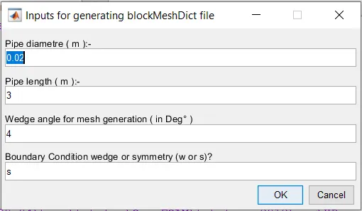
The blockMeshDict file generated, uses macro expansion ($) which expands the value of a variable defined earlier in the file and #eval directive to calculate co-ordinates in inline expressions.
/*--------------------------------*- C++ -*----------------------------------*
| =========                 |                                                 |
| \      /  F ield         | OpenFOAM: The Open Source CFD Toolbox           |
|  \    /   O peration     | Version:  v2012                                 |
|   \  /    A nd           | Website:  www.openfoam.com                      |
|    \/     M anipulation  |                                                 |
*---------------------------------------------------------------------------*/
FoamFile
{
    version     2.0;
    format      ascii;
    class       dictionary;
    object      blockMeshDict;
}
// * * * * * * * * * * * * * * * * * * * * * * * * * * * * * * * * * * * * * //

scale   1;
// Inputs

r 0.01;              // Radius (m)
L 3;                 // Length of pipe (m)
theta 4;             // Wedge angle (in degree)
a  ($theta)*3.142/180;     // theta in radians

//............................Calculating Co-ordinates
x1 #eval {-sin($a/2)*$r};
y1 #eval {cos($a/2)*$r};
x2 #eval {sin($a/2)*$r};
y2 #eval {cos($a/2)*$r};
//............................Calculating interpolating co-ordianates
xi 0;
yi $r;

vertices
(
    (0 0 0)          //0
	($x1 $y1 0)      //1
	($x2 $y1 0)      //2

    (0 0 $L)         //3
	($x1 $y1 $L)     //4
	($x2 $y1 $L)     //5
);

blocks
(
   hex (0 3 5 2 0 3 4 1) (500 30 1) simpleGrading (1 0.4 1)
);

edges
(
   arc 2 1 ($xi $yi 0)
   arc 5 4 ($xi $yi $L)
);

boundary
(
	inlet
    {
        type patch;
        faces
        (
            (0 2 1 0)
        );
    }

	outlet
    {
        type patch;
        faces
        (
			(3 5 4 3)
        );
    }

	fixedWalls
    {
        type wall;
        faces
        (
            (1 4 5 2)
        );
    }

    front
    {
        type symmetry; //keyword "wedge" in HPpipe_W/system/blockMeshDict
        faces
        (
            (0 3 4 1)
        );
    }

	back
    {
        type symmetry;
        faces
        (
			(0 3 5 2)
        );
    }

	axis
	{
		type empty;
		faces
		(
		    (0 3 3 0)
		);
	}
);

mergePatchPairs
(
);

// ************************************************************************* //
# Initial conditions :
Transport properties :-
The constant folder contains transport properties that should be defined before simulation. We will set transport model as "Newtonian" & define kinematic viscosity as `nu=1.004"x"10^(−6)" "m^2//s`
/*--------------------------------*- C++ -*----------------------------------*
| =========                 |                                                 |
| \      /  F ield         | OpenFOAM: The Open Source CFD Toolbox           |
|  \    /   O peration     | Version:  v2012                                 |
|   \  /    A nd           | Website:  www.openfoam.com                      |
|    \/     M anipulation  |                                                 |
*---------------------------------------------------------------------------*/
FoamFile
{
    version     2.0;
    format      ascii;
    class       dictionary;
    location    "constant";
    object      transportProperties;
}
// * * * * * * * * * * * * * * * * * * * * * * * * * * * * * * * * * * * * * //

transportModel  Newtonian;

nu             [ 0 2 -1 0 0 0 0 ] 1.004E-6;


// ************************************************************************* //
U (velocity vector) :-
Initial conditions of U are located in 0/U. For laminar flow the initial velocity should be `U = 0.105" "m//s^2` along z-direction i.e pipe length. The U (velocity vector) file should be modified as shown,
/*--------------------------------*- C++ -*----------------------------------*
| =========                 |                                                 |
| \      /  F ield         | OpenFOAM: The Open Source CFD Toolbox           |
|  \    /   O peration     | Version:  v2012                                 |
|   \  /    A nd           | Website:  www.openfoam.com                      |
|    \/     M anipulation  |                                                 |
*---------------------------------------------------------------------------*/
FoamFile
{
    version     2.0;
    format      ascii;
    class       volVectorField;
    object      U;
}
// * * * * * * * * * * * * * * * * * * * * * * * * * * * * * * * * * * * * * //

dimensions      [0 1 -1 0 0 0 0];

internalField   uniform (0 0 0);

boundaryField
{
    inlet
    {
        type            fixedValue;
        value           uniform (0 0 0.105);
    }

	outlet
    {
        type            zeroGradient;
    }

	fixedWalls
    {
        type            noSlip;
		value           uniform (0 0 0);
    }

    front
    {
        type            symmetry; //keyword "wedge" in HPpipe_W/system/blockMeshDict
    }

	back
    {
        type            symmetry;
    }

	axis
	{
		type  			empty;
	}
}

// ************************************************************************* //
p (pressure):-
Initial conditions of U are located in 0/U. All the incompressible solvers implemented in OpenFOAM, use the modified pressure, that is,
`" "p = P/rho" "m^2s^(-2)`
This pressure will be multiplied with density during post-processing to get actual pressure in Pa. The p (pressure) file should be modified as shown,
/*--------------------------------*- C++ -*----------------------------------*
| =========                 |                                                 |
| \      /  F ield         | OpenFOAM: The Open Source CFD Toolbox           |
|  \    /   O peration     | Version:  v2012                                 |
|   \  /    A nd           | Website:  www.openfoam.com                      |
|    \/     M anipulation  |                                                 |
*---------------------------------------------------------------------------*/
FoamFile
{
    version     2.0;
    format      ascii;
    class       volScalarField;
    object      p;
}
// * * * * * * * * * * * * * * * * * * * * * * * * * * * * * * * * * * * * * //

dimensions      [0 2 -2 0 0 0 0];

internalField   uniform 0;

boundaryField
{
    inlet
    {
        type            zeroGradient;
    }

	outlet
    {
        type            fixedValue;
        value           uniform 0;
    }

    fixedWalls
    {
        type            zeroGradient;
    }

    front
    {
        type            symmetry; //keyword "wedge" in HPpipe_W/system/blockMeshDict
    }

	back
    {
        type            symmetry;
    }

	axis
	{
		type  			empty;
	}
}

// ************************************************************************* //
# Solving :
We will use icoFoam solver as done previously and the same controlDict file for simulation of our case.
# Validation of results :
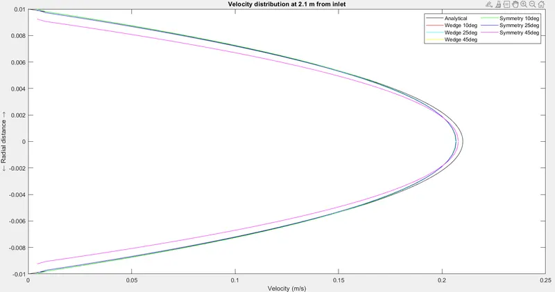
- It can be seen that the velocity profile becomes fully developed after 2.1 m from inlet. This can be verified by checking the error in velocity from analytical profile as done in code below.
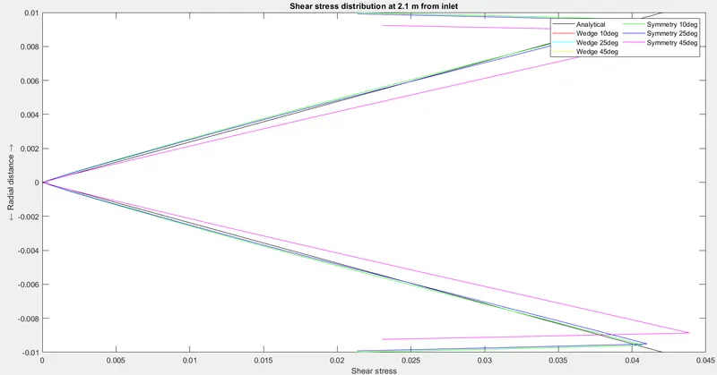
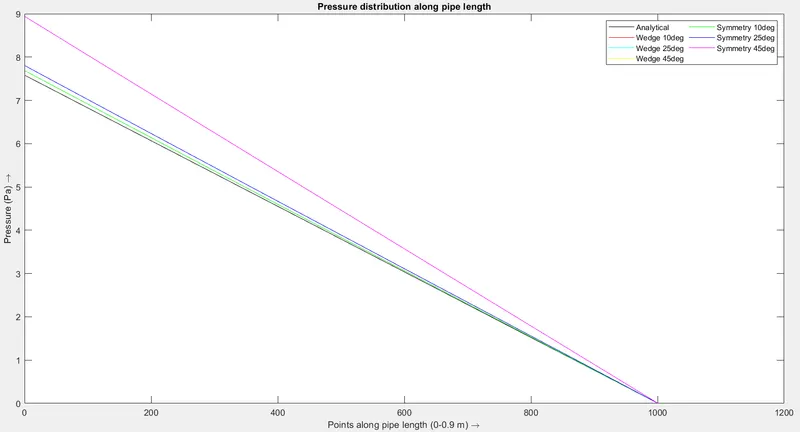
- We will import pressure data "Dy_pressure", velocity data "U_Magnitude" & shear stress data "tau_Magnitude" from paraview in .txt format and then read it using readmatrix() in the MATLAB code for comparing pressure, velocity & shear stress profiles.
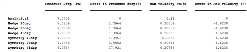
- Next the results will be plotted and errors will be computed.
MATLAB code for Validating Numerical results
clearvars
close all
clc

% MATLAB code for validating results with Hagen-Poiseuille equations
% Inputs
D = 0.02;
R = D/2;
L = 0.9;                                   % Pipe length in FDF region = 3 - 2.1 = 0.9 m
r = linspace(-R,R,1001);
mu = 1.002*10^-3;
Uavg = 0.105;

% Calculating analytical values
Umax = 2*Uavg;
dPdL = -32*mu*Uavg/(D^2);
P    = abs(dPdL*linspace(L,0,1001));       % Magnitude of Pressure
U    = abs((1/(4*mu))*dPdL*(R^2 - r.^2));  % Magnitude of velocity
tau  = abs((abs(r)/2)*dPdL);               % Magnitude of shear stress

% Reading numerically computed data
strAry = ["W10" "W25" "W45" "S10" "S25" "S45"];
[tau_N,U_N,P_N] = deal(zeros(1,1001));

for i = 1:length(strAry)
    str1 = "u_tau_2_1_"+strAry(i)+".txt";
    str2 = "p_Dy_lastTimeStep_"+strAry(i)+".txt";

    M          = readmatrix(str1);
    tau_N(i,:) = abs(M(:,5));
    U_N(i,:)   = M(:,3);
    P_N(i,:)   = readmatrix(str2);
end

LgdName = ["Analytical" "Wedge 10deg" "Wedge 25deg" "Wedge 45deg"...
               "Symmetry 10deg" "Symmetry 25deg" "Symmetry 45deg"];
pColor = ["r" "c" "y" "g" "b" "m"];

% Validating numerical FDF with analytical FDF
figure('Position',[100 100 560 420])
plot(U,r,'k')
hold on
for i = 1:length(strAry)
    plot(U_N(i,:),r,pColor(i))
end
xlabel('Velocity (m/s)')
ylabel('leftarrow Radial distance rightarrow')
legend(LgdName,'NumColumns',2)
title('Velocity distribution at 2.1 m from inlet')

% Validating numerical S.S. with analytical S.S.
figure('Position',[660 100 560 420])
plot(tau,r,'k')
hold on
for i = 1:length(strAry)
    plot(tau_N(i,:),r,pColor(i))
end
xlabel('Shear stress')
ylabel('leftarrow Radial distance rightarrow')
legend(LgdName,'NumColumns',2)
title('Shear stress distribution at 2.1 m from inlet')

% Validating numerical pressure drop with analytical pressure drop
figure()
plot(P,'k')
hold on
for i = 1:length(strAry)
    plot(P_N(i,:),pColor(i))
end
xlabel('Points along pipe length (0-0.9 m) rightarrow')
ylabel('Pressure (Pa) rightarrow')
legend(LgdName,'NumColumns',2)
title('Pressure distribution along pipe length')

% Calculating errors in pressure drop and max velocity
P_drp(1,1) = P(1,1)-P(1,end);
Max_U(1,1) = max(U);
error_P(1,1) = 0;
error_U(1,1) = 0;

for i = 1:6
    P_drp(i+1,1) = P_N(i,1) - P_N(i,end);
    Max_U(i+1,1) = max(U_N(i,:));
    error_P(i+1,1) = 100*(P_drp(i+1,1) - P_drp(1,1))/P_drp(1,1);
    error_U(i+1,1) = 100*(Max_U(1+1,1) - Max_U(1,1))/Max_U(1,1);
end

t1 = table(P_drp,error_P,Max_U,error_U,...
          'variableNames',["Pressure Drop (Pa)","Error in Pressure drop(%)",...
           "Max Velocity (m/s)","Error in Max velocity (%)"],...
          'rowNames',LgdName);
disp(t1)

% END OF PROGRAM
Outputs
# Inferences :
- We can see that the velocity & shear stress profiles match closely with analytical profiles in case of wedge BC while the profiles deviate slightly with symmetry BC.
- The pressure profiles see major deviation with increasing angle in case of symmetry BC and the error in pressure drop becomes `~18%` with `45deg` angles.
- So for higher wedge angles wedge BC gives more accurate pressure drop.