Flow over a Cylinder.

# Objective:

To simulate the flow over a cylinder.

# Introduction:

In this project, we are going to simulate vortex shedding observed in the case of flow over a cylindrical surface using different Reynolds numbers from `10` to `10^5`. We will carry out qualitative analysis for this and hence will use a steady-state solver except for Reynolds’s no. 100 we will use a transient solver for quantitative analysis.

# Theory:

Cylindrical surfaces are commonly encountered in many applications interacting with fluid flows like bridges, cables, buildings, etc and hence predicting the flow over these surfaces is of prime importance.

Although the object of study has a simple geometry the flow over it is complicated and varies with Reynolds‘s number.

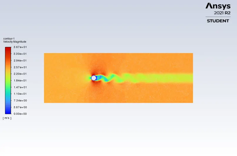
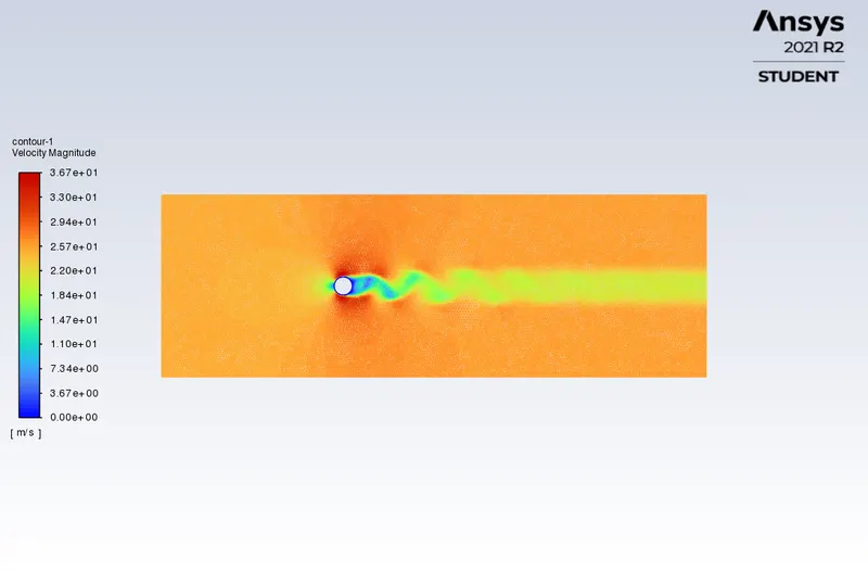
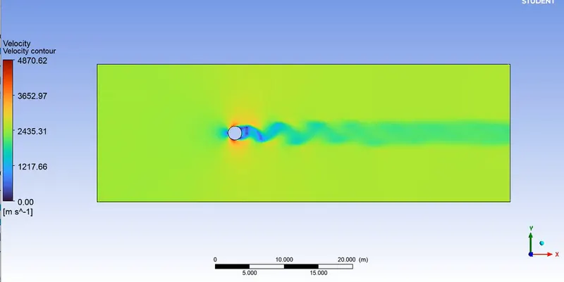
Von Karman vortex street is a repeating pattern of swirling vortices, caused by a process known as vortex shedding. Vortex shedding is an oscillating flow that takes place when a fluid such as air or water flows past a bluff (as opposed to a streamlined) body at certain velocities, depending on the size and shape of the body.

The fluid flow past the object creates alternating low-pressure vortices on the downstream side of the object. The object will tend to move toward the low-pressure zone. If the bluff structure is not mounted rigidly and the frequency of vortex shedding matches the resonance frequency of the structure, then the structure can begin to resonate, vibrating with harmonic oscillations driven by the energy of the flow.

Governing equation:
The frequency at which vortex shedding takes place for an infinite cylinder is related to the Strouhal number by the following equation: `" "St = (fD)/U`

Where St is the dimensionless Strouhal number, `f` is the vortex shedding frequency, `D` is the diameter of the cylinder `(m)`, and `U` is the flow velocity `(m\s)`.

# Geometry & Meshing:

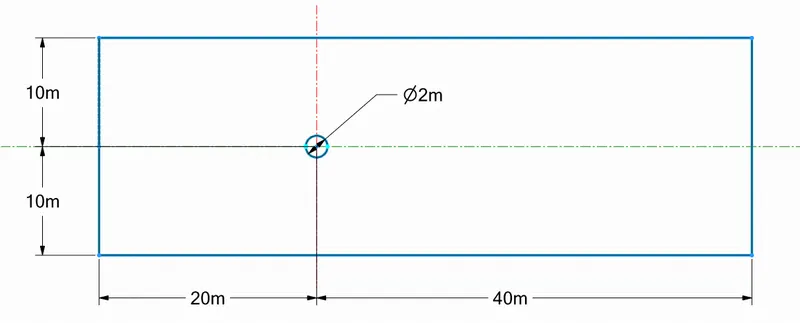
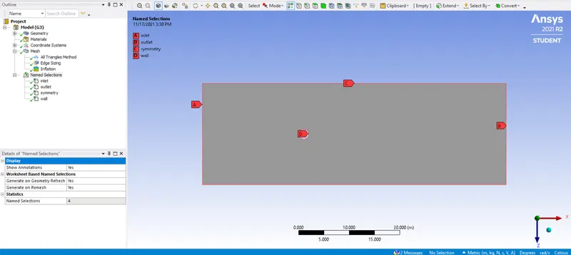
• The geometry is a sheet of 60×20 m with a hole (at (0,0)) which represents a cylinder in the 2D plane. The hole diameter is (D =) 2 m with a margin from domain boundaries of 20D from the fluid inlet, 40D from the outlet, and 10D from the top boundary as shown below.

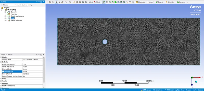
• The fine mesh is made of triangular elements with an element size of 0.25 m.

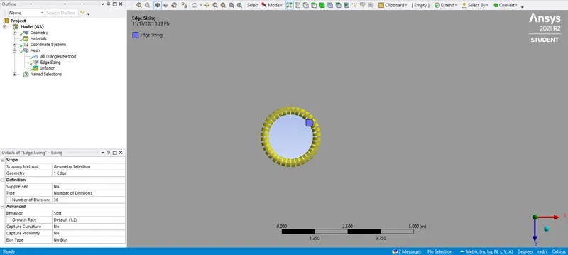
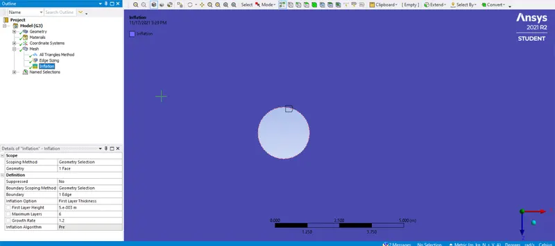
• Next, the region near the hole (cylinder) needs to be refined further as flow physics changes near the cylinder wall. This is done using element sizing on a circular edge with 36 divisions as shown.

• An inflation layer is added near the cylinder (hole) for an even finer mesh with the settings shown below.

• During mesh generation, edges are named so that Fluent can automatically recognize & set the appropriate types of boundary conditions.

# Setting up the case:

• The below-mentioned case setup is the same for all simulations discussed in PART-I & PART-II with only minor changes.
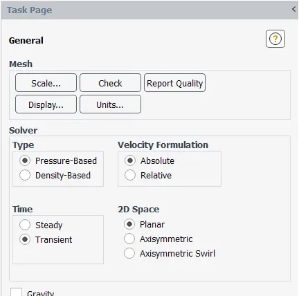
• For simulating the flow we will use the steady-state solver to capture the flow physics but for frequency analysis (FFT) we will use a transient solver for a time-wise accurate solution.
• Also for varying Reynolds no. we will just vary the flow velocity from the inlet.

(1) Solver settings:

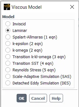
(2)Vicous model set to laminar

(3) Creating custom fluid for ease of analysis.

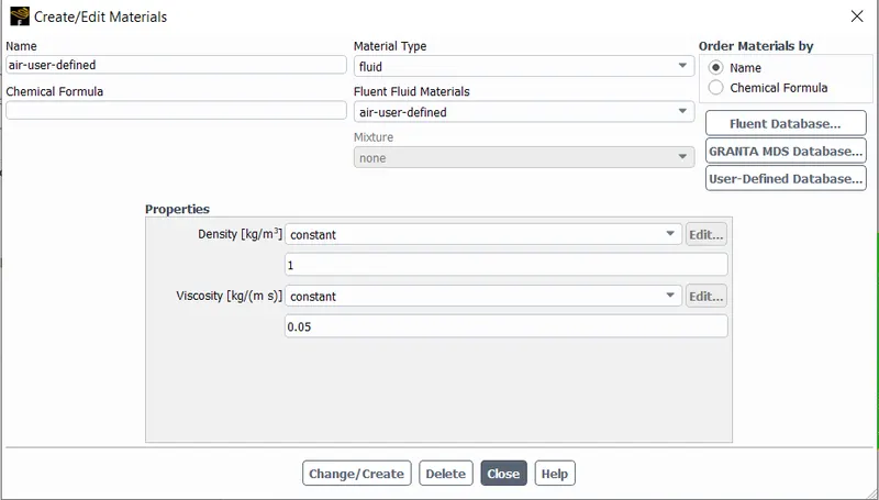
(4)Setting custom fluid in domain

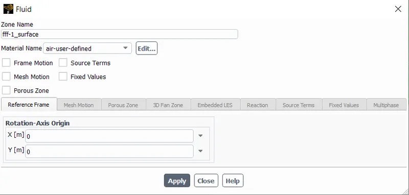
(5) Applying boundary values

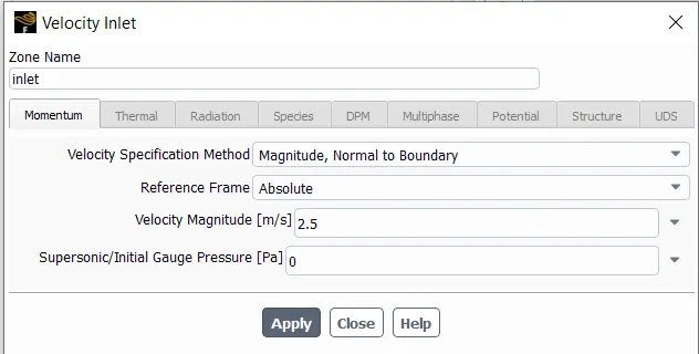
(6) Setting reference values from inlet

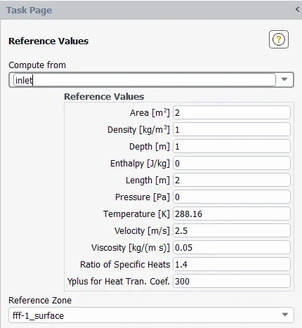
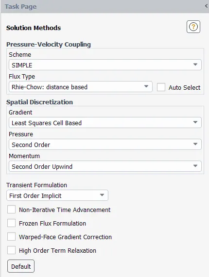
(7) Solution methods & discretization

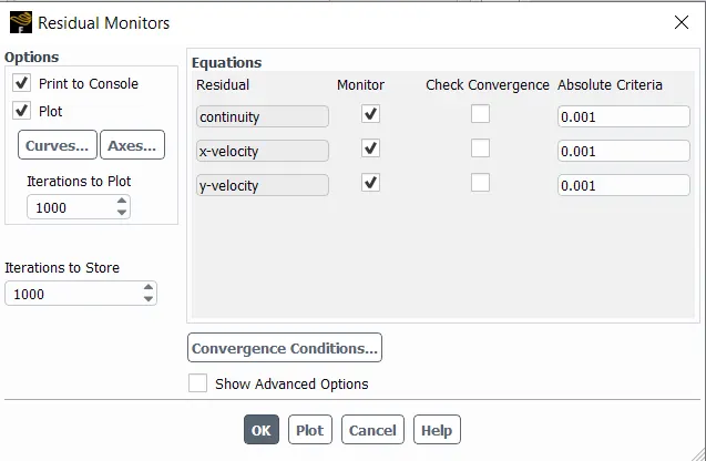
(8) Removing convergence criteria so that solution wiggles can be monitored for set no. of iterations.

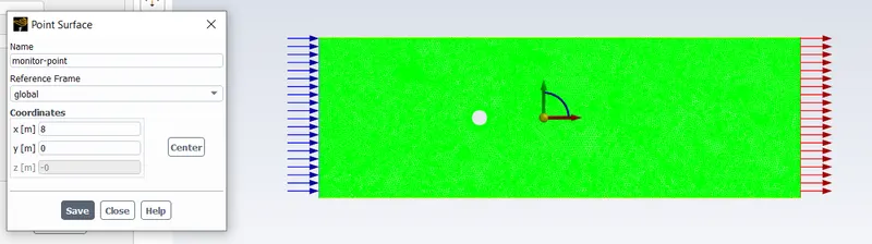
(8) Generating monitor point

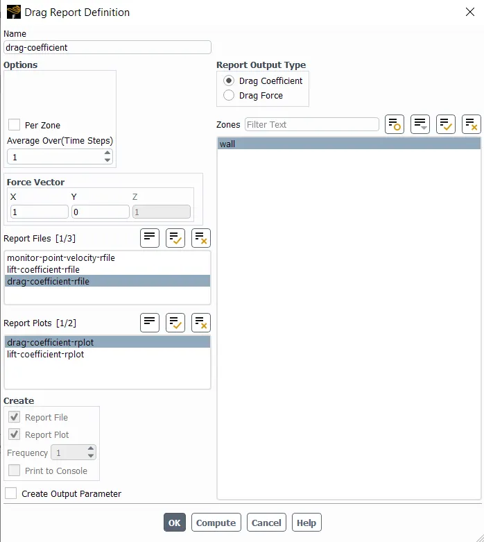
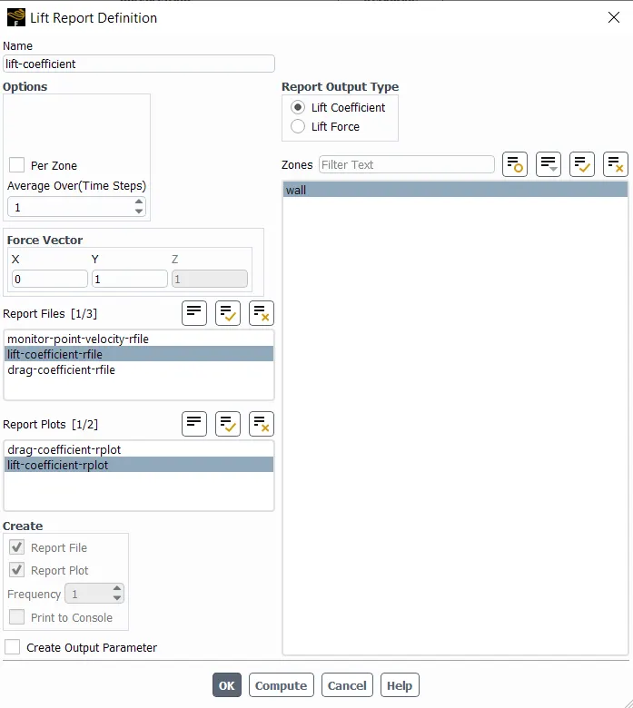
(9) Report definitions:

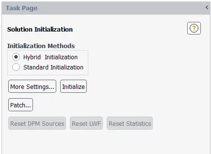
(10) Initializing the solution:

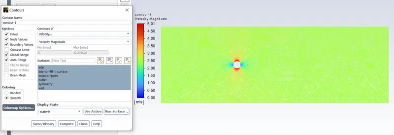
(11) Generating velocity contour of the entire domain (below figure shows initial velocity field).

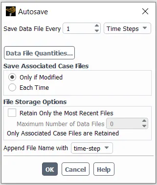
(12) Enabling austosave for solution visualization in CFD-Post.

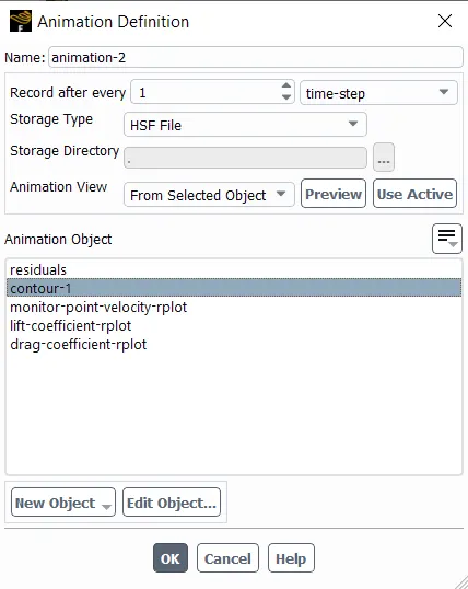
(13) Creating animation for visualization in fluent.

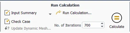
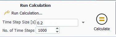
(14) Setting no. of iterations and time step size (for transient solver)

PART-I: Simulating the flow with the steady and unsteady case and calculating the Strouhal Number for Re= 100.

For both, the cases inlet velocity will be set to 2.5 m/s so that Reynolds no. is,

`" "Re = ((1)(2.5)(2))/((0.05)) = 100`

Case 1: Steady-state solver

Inferences:

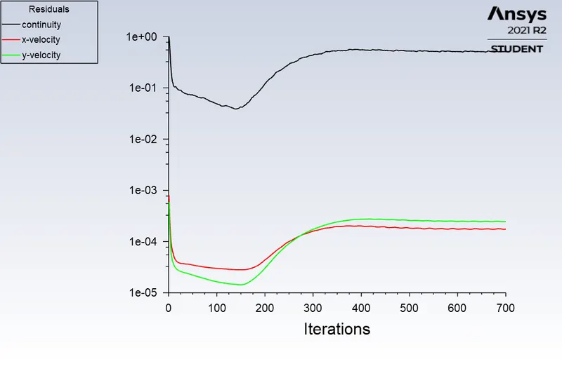
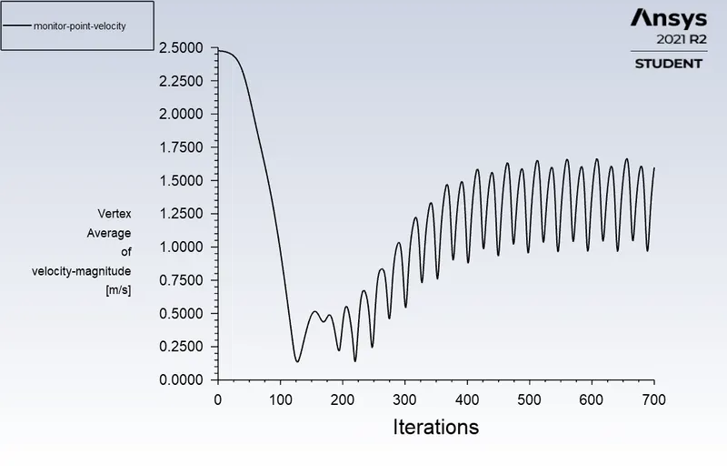
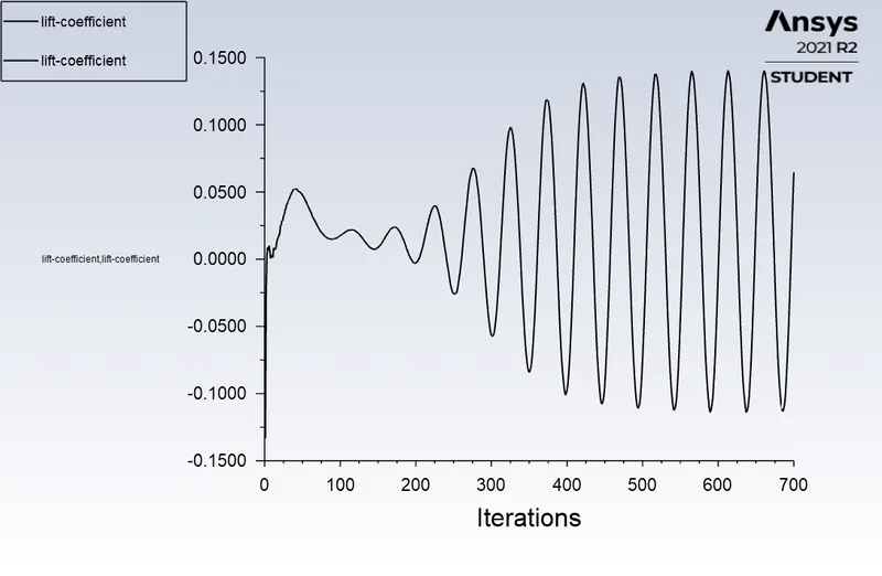
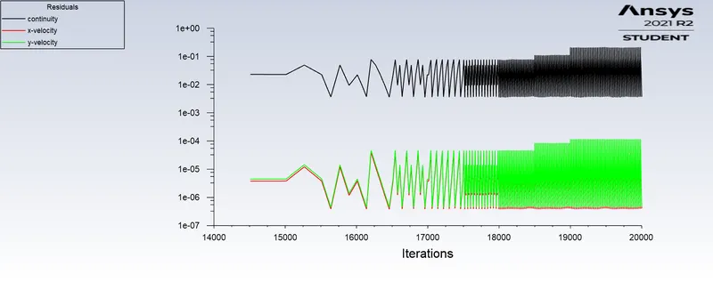
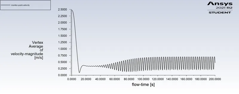
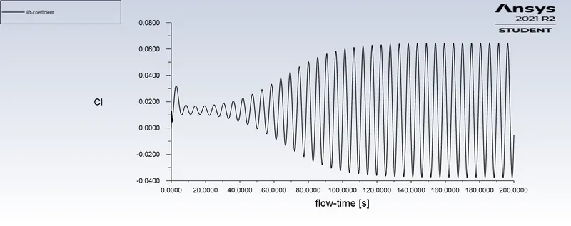
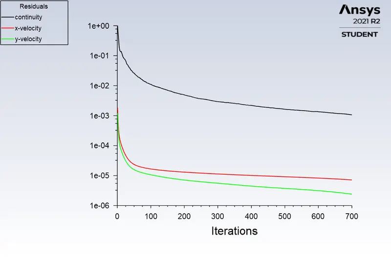
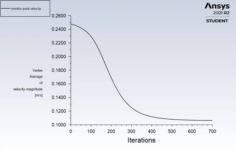
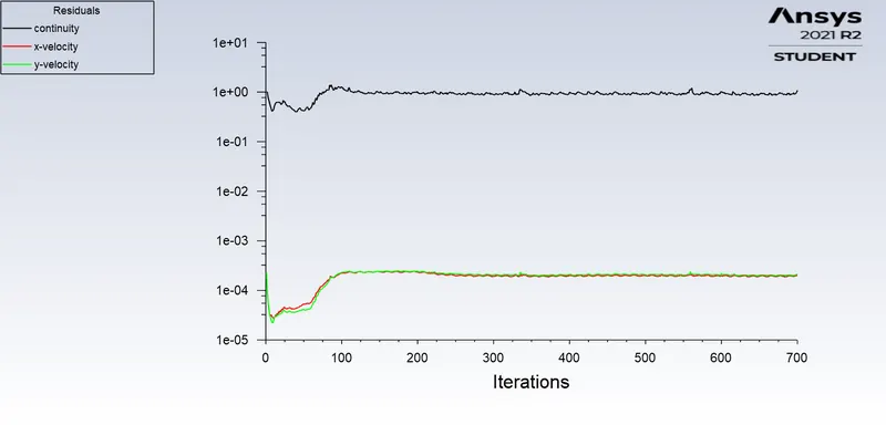
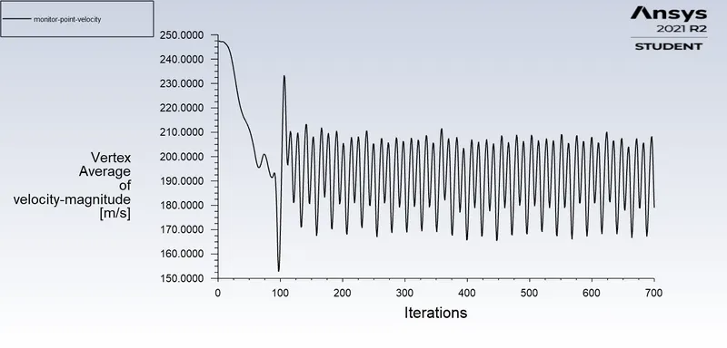
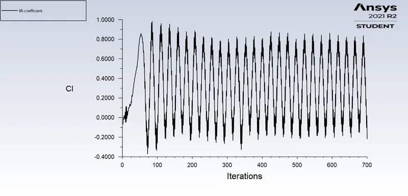
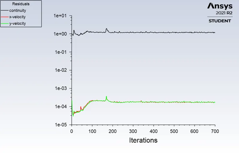
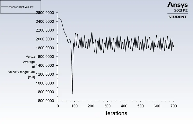
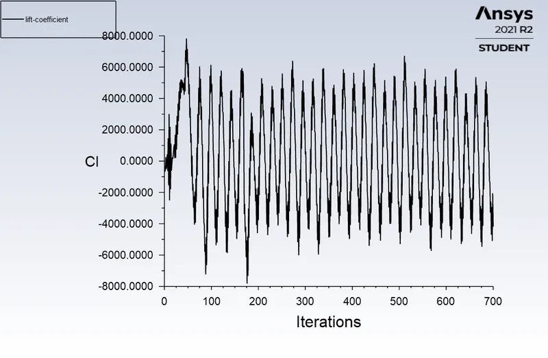
• We can see that the residuals are converged to a nearly straight line with a repeating pattern but the monitor point velocity and lift coefficient are oscillating.
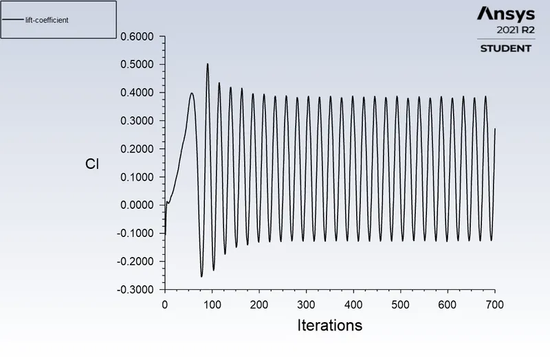
• This indicates that vortex shedding is taking place causing fluctuations in direction of lift force on the cylinder. The velocity variation in the wake (monitor point velocity plot) also confirms this.
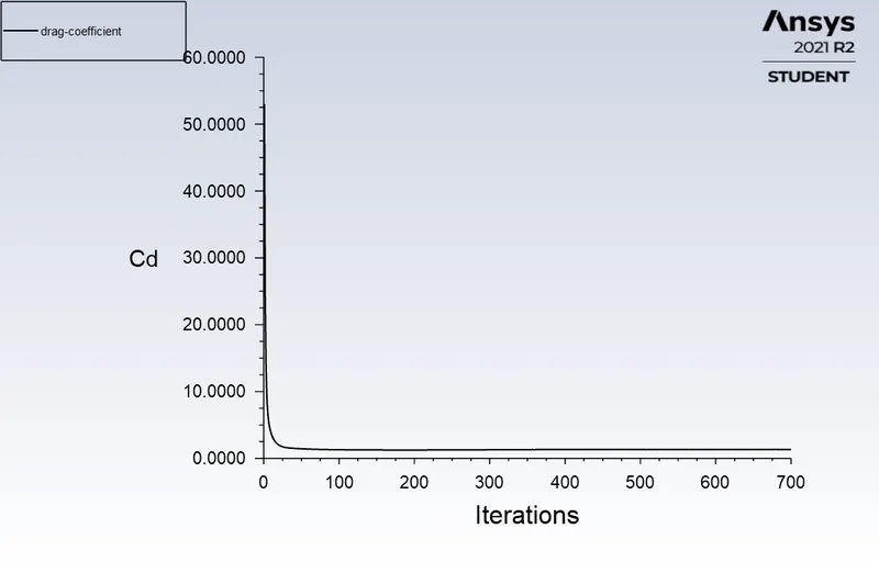
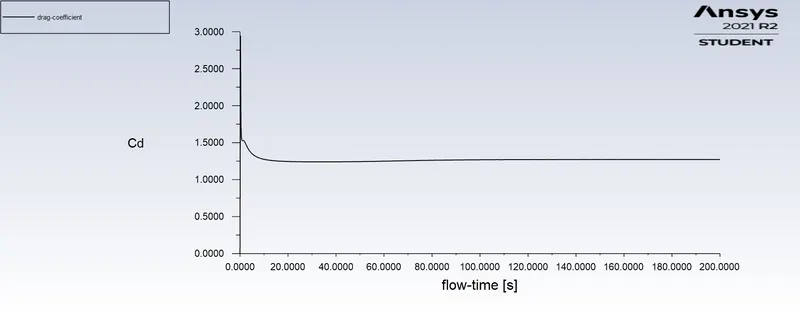
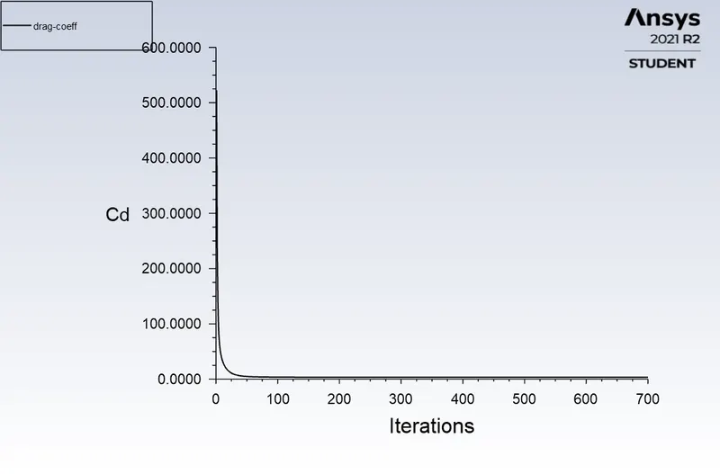
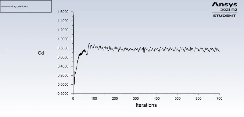
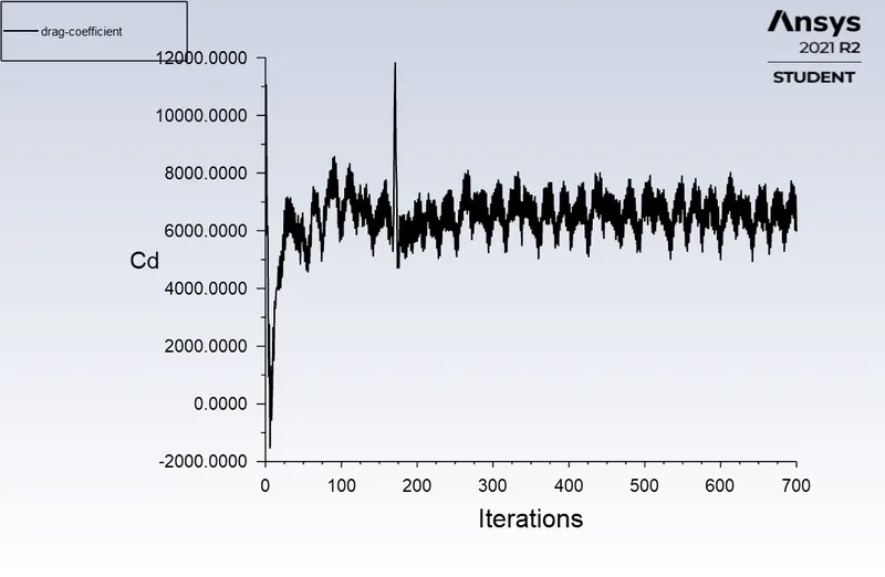
• The drag force remains nearly a straight line because the horizontal component of velocity on the cylinder stays the same.
• Hence we have captured the physics of the flow and the solution has converged.
• The animation below shows the flow development through the iterations.

Case 1: Unsteady-state solver

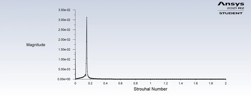
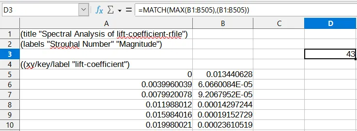
• The strouhal no. for the simulation can be found by reading the CSV file from FFT analysis in excel.
• There are two columns first is strouhal no. and the second is magnitude. The following command finds the index in column B (magnitude) where the magnitude is maximum.

  =MATCH(MAX(B1:B505),(B1:B505))

Inferences:

• Similar results are obtained as were in the case of steady-state solver hence the solution is converged.
• This simulation uses a transient solver which is time-wise accurate and hence shows actual flow variation with time.
• The strouhal no. for the simulation is `Sr =0.15185`.
• The animation below shows the flow development through the time steps.

PART-II: Calculate the coefficient of drag and lift over a cylinder by varying the Reynolds number from `10` to `10^5`

CASE 1 : Re = 10 ,(inlet velocity = 0.25 m/s)

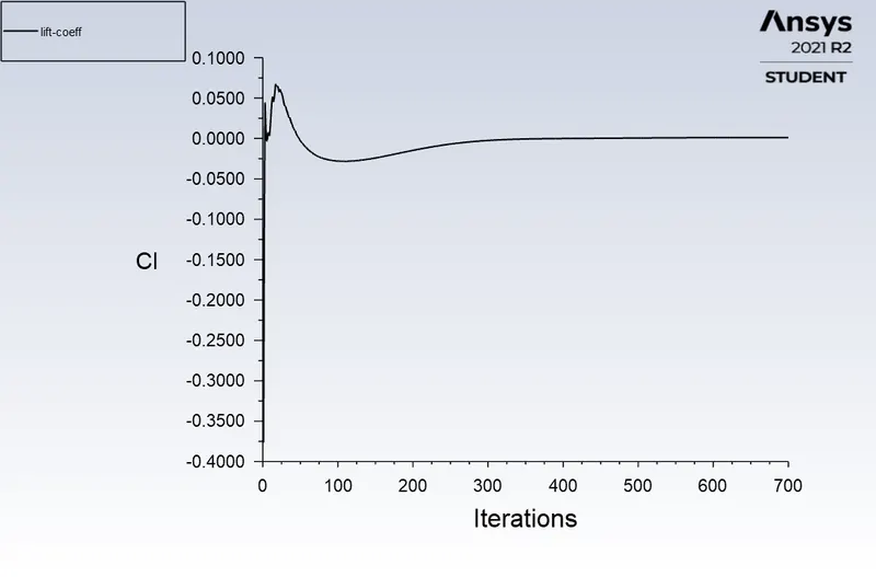
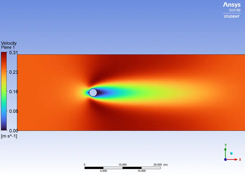
CASE 2 : Re = 100 ,(inlet velocity = 2.5 m/s)

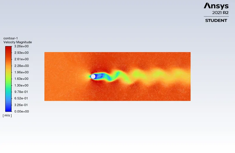
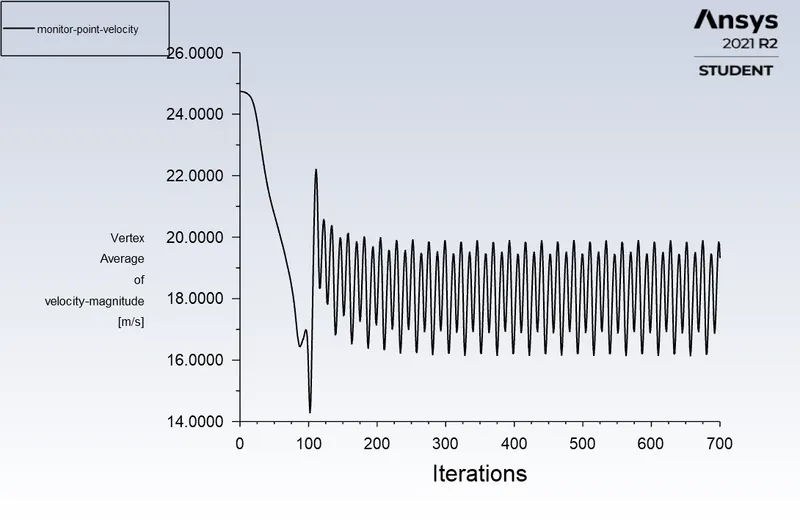
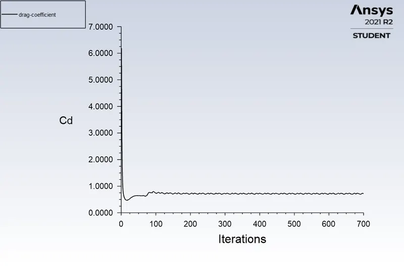
CASE 3 : Re = 1000 ,(inlet velocity = 25 m/s)

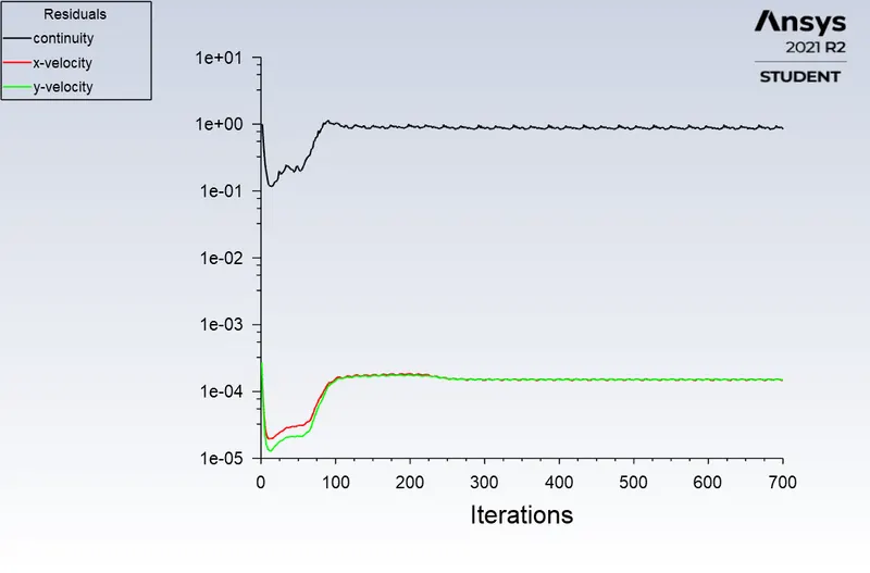
CASE 4 : Re = 10^4 ,(inlet velocity = 250 m/s)

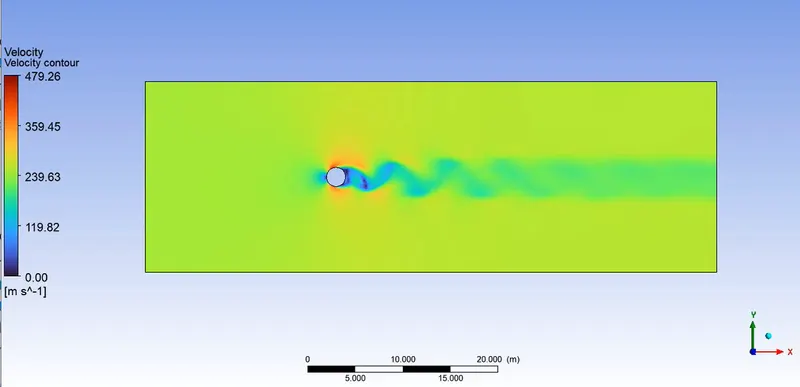
CASE 5 : Re = 10^5 ,(inlet velocity = 2500 m/s)

# Results:

Reynolds Number	Coefficient of Drag (`C_D`)
`10^1`	3.3252711
`10^2`	1.3366145
`10^3`	0.72887913
`10^4`	0.7380259
`10^5`	0.59680406

# Inferences:

• It can be seen that the drag coefficient reduces with increasing Reynolds Number.
• For flow with Re 10, there is no flow separation & hence karman vortex street is not observed.
• The `C_D` computed at Re 10 can be validated with the value published in [1] which is `C_D = 1.3353` the absolute error is `0.13 %`.

References:

[1] https://www.sciencedirect.com/science/article/pii/S0307904X08000243