Simulating Rayleigh Taylor Instability
The Rayleigh–Taylor instability, or RT instability (after Lord Rayleigh and G. I. Taylor), is the instability of an interface between two fluids of different densities which occurs when the lighter fluid is pushing the heavier fluid. Examples include the behavior of water suspended above oil in the gravity of Earth, mushroom clouds like those from volcanic eruptions and atmospheric nuclear explosions
Some CFD models based on Rayleigh-Taylor instability:-
1)Kelvin-Helmholtz instability:
This is the kind of instability that occurs when there is velocity shear in a single continuous fluid or a velocity difference across the interface between two fluids. Winds blowing over water bodies is an excellent example of this kind of instability.
2)Richtmyer–Meshkov instability:
Richtmyer–Meshkov instability is the fluid flow phenomenon that occurs when a shock wave impinges (in the normal direction) upon an interface separating two gases having different densities. The instability causes perturbations on the interface to grow, producing vortical structures which potentially result in a turbulent mixing layer.
3)Plateau–Rayleigh instability:
The Plateau–Rayleigh instability, often just called the Rayleigh instability, explains why and how a falling stream of fluid breaks up into smaller packets with the same volume but less surface area. The driving force of this instability is that liquids, by virtue of their surface tensions, tend to minimize their surface area. It is related to the Rayleigh–Taylor instability and is part of a greater branch of fluid dynamics concerned with fluid thread breakup.
Simulation of Rayleigh-Taylor instability:
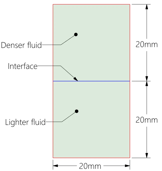
The 2D simulation setup consists of 20x20 mm computational domains of air and water as shown in figure 1. The interface is the shared topology which is a straight line initially. The coarse & fine meshes are made up completely of hexahedral cells with an element size of 0.5 mm & 0.2 mm respectively.
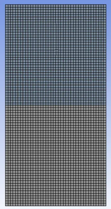
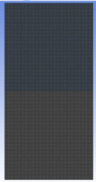
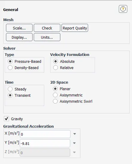
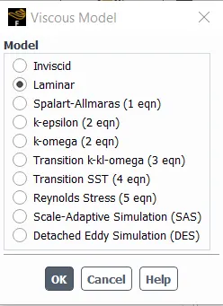
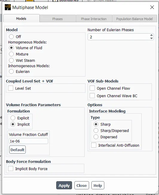
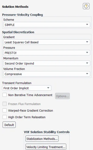
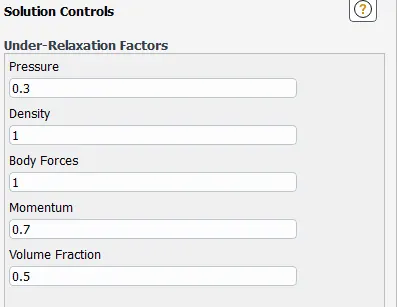
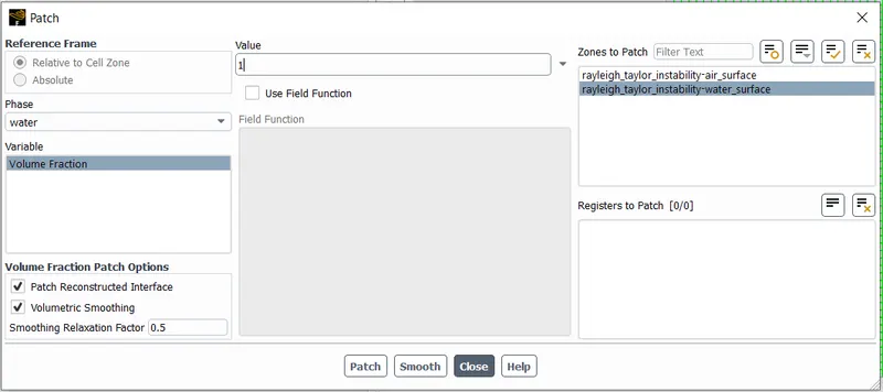
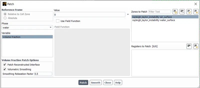
The flow is assumed to be laminar with gravity force downwards. The volume of Fluid (VOF) method is used with an implicit numerical scheme. The volume fraction is patched as 1 for water and 0 for air after standard initialization.
Transient simulations are carried out with a time step size of 0.005 for 1000 iterations so, the simulation time is 5 seconds.
CASE I:- Water & air
Coarse mesh (element size 0.5 mm),
https://drive.google.com/file/d/13B6vlcRtFLK_JznQGTRujDj5KIe5M5f2/view?usp=sharing
The simulation was performed again with a refined mesh (element size 0.2 mm) & the results are below.
https://drive.google.com/file/d/19Ny3Uy2HHvHe0L_EszOoWamRWsZk94Q7/view?usp=sharing
CASE II:- Water & user-defined fluid
The same solver settings were used but a much denser and viscous fluid was placed below water.
https://drive.google.com/file/d/1fTWM6J_QNMubXxlwNRH8pOGY_GmYiwTE/view?usp=sharing
Inferences:
Transient simulations
Since we are interested in observing the time-wise variations in the domain after the onset of perturbation, transient simulation is chosen. This is so because steady-state simulations are not time-wise accurate in spite of being faster. Also, fluids physics dictate that the lighter fluid will float over heavier (denser) fluid which makes steady-state simulations meaningless.
Mesh refinement
Mesh refinement was done because coarser mesh means the region between the elements needs to be interpolated. This gives sufficiently accurate flow fields when flow variation is low however for large flow variations inaccuracies develop due to flow variations between the elements. If the mesh is too coarse, the simulation results might be inaccurate or sometimes even unphysical.
Atwood number
The Atwood number is a dimensionless number in fluid dynamics used in the study of hydrodynamic instabilities in density stratified flows. Mathematically, it is the difference in the fluid densities divided by their sum.
`A = (rho_1 – rho_2)/(rho_1 + rho_2)`
`A ="Atwood number"` `"(dimensionless)"`
`ρ_1="Density of heavier fluid"` `(kg//m^3)`
`ρ_2="Density of lighter fluid"` `(kg//m^3)`
For Water-Air interface,
`rho_1 = 998.2` `kg//m^3` (water)
`rho_2 = 1.225` `kg//m^3` (air)
`therefore A = 0.998`
For Water & hypothetical fluid interface,
`rho_1 = 998.2` `kg//m^3` (water)
`rho_2 = 400` `kg//m^3` (air)
`therefore A = 0.4`
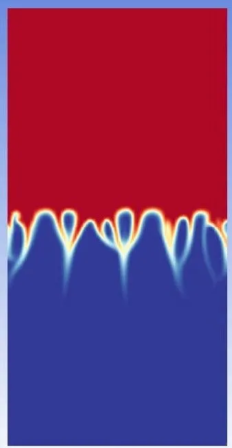
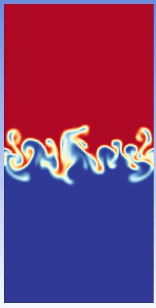
Atwood number is an important parameter in the study of Rayleigh–Taylor instability. For Atwood number close to 0, RT instability flows take the form of symmetric “fingers” of fluid; for Atwood number close to 1, the much lighter fluid “below” the heavier fluid takes the form of larger bubble-like plumes.
Hence for CASE I fingers of fluid are formed in fluid while in CASE II, plumes are observed as shown below.
(a) "Fingers" (b)"Plumes"
figure: RT instabilty behaviour of (a) Water-air & (b) Water-UD fluid