Finding species concentrations using multivariate Newton Rhapson Solver

Theory:

In the combustion mechanism, the rate of change of concentration i.e. the rates of production or depletion of different species are governed by a system of coupled ODEs. Also, it is not uncommon to see the concentration of some species changing rapidly while others in change comparatively slowly. Hence these systems are coupled stiff ODEs.

The following set of coupled ODEs are stiff and are a good representation of reaction rates in a combustion mechanism,

`" "dy_1/dt = -0.04y_1 + 10^4y_2y_3`

`" "dy_2/dt = 0.04y_1 - 10^4y_2y_3 - 3*10^7y_2^2`

`" "dy_3/dt = 3*10^7y_2^2`

These coupled ODEs cannot be solved through integration easily and hence numerical integration is needed. For this project, we will solve the above ODEs using the multivariate Newton-Raphson method. It is an extension of the univariate Newton-Raphson method,

`" "y_n = y_("guess") - alpha*[f(y_("guess"))/f^(')(y_("guess"))]" "("Univariate NR method")`

`" "Y_n = Y_("Guess") - alpha*(J^-1)*(F)" "("Multi-variate NR method")" ...(1)"`

Where,

`" "Y_("Guess") = "Guessed value(s) matrix from previous iteration"`

`" "J = "Jacobian of coupled ODEs"`

`" "F = "Function matrix which needs to be solved"`

The N-R method is essentially a root-finding algorithm for a homogenous equation so, the above ODEs need to be converted to a system of homogenous equations.

Discretization

Since we are using time stepping, the time derivatives will be discretized using backward differencing,

`" "((y_1^n - y_1^(n-1))/(Delta t)) = -0.04y_1 + 10^4y_2y_3`

`" "((y_2^n - y_2^(n-1))/(Delta t))= 0.04y_1 - 10^4y_2y_3 - 3*10^7y_2^2`

`" "((y_3^n - y_3^(n-1))/(Delta t)) = 3*10^7y_2^2`

Homogenizing

Let `h = Delta t` and `n` denote the current time level,

`" "f_1^n = y_1^(n-1) + h*(-0.04*y_1^n + 10^4*y_2^n*y_3^n) - y_1^n = 0`

`" "f_2^n = y_2^(n-1) + h*(0.04*y_1^n - 10^4*y_2^n*y_3^n - 3*10^7*(y_2^n)^2) - y_2^n = 0`

`" "f_3^n = y_3^(n-1) + h*(3*10^7*(y_2^n)^2) - y_3^n = 0`

These functions will be represented by function vector F as,

`" "F = [[f_1^n], [f_2^n], [f_3^n]]`

Jacobian

The jacobian is defined as,

`" "J = [ [(del f_1)/ (del y_1), (del f_1)/ (del y_2), (del f_1)/ (del y_3)], [(del f_2)/ (del y_1), (del f_2)/ (del y_2), (del f_2)/ (del y_3)], [(del f_3)/ (del y_1), (del f_3)/ (del y_2), (del f_3)/ (del y_3)] ]`

Each partial space derivative will be numerically computed using first-order backward differencing e.g.,

`" "(del f_1)/(del y_1) = (f_1(y_1, y_2, y_3) - f_1(y_1 - Delta y_1, y_2, y_3))/ (Delta y_1)`

Initial guess

The guess values for `t=0` will be represented by vector `Y_("Guess")` as,

`" "Y_("Guess") = [ [1], [0], [0] ]`

Relaxation

Relaxation factor `alpha` will be set to `1` and left as it is unless the solution plot shows wiggles.

Coding Approach:

1. First three functions representing `f_1, f_2 & f_3` are defined.
2. For finding the partial derivative, `"fprime()"` is defined which finds all partial derivatives of function `f` for each `y`.
3. The function `"jacobian()"` calls `"fprime()"` three times with `f_1(), f_2() & f_3()` and fills the values in `1st, 2nd & 3rd` rows respectivly.
4. Next, no. of time-steps `"n_ts"` are computed from time interval `"(t, tend)"`.
5. The time step size is used to pre-allocate array `"Y"` (for speed) and set bounds for `"for"` time loop.
6. Next, `"Y_(Guess)"` is initialized with guess values for `t=0` and a copy is passed to `"F"` to initialize it as well.
7. In the time loop, the initial error & tolerance value for a converged solution is set first.
8. In the convergence loop, equation `"(1)"` is used to find an iterative solution of `"Y"` for the time-step.
9. At the end of the time loop, the computed time-step value is assigned to `"Y[t]"` and the process is repeated.
10. At last, the results are plotted.

#%% FUNCTION DEFINITIONS
import time
from math import floor
import numpy as np
from   numpy.linalg import inv
import matplotlib.pyplot as plt
from copy import deepcopy

def f1(y1_prev: float, y1: float, y2: float, y3: float, h: float) -> np.ndarray:
    return y1_prev + h*(-0.04*y1 + (10**4)*y2*y3) - y1

def f2(y2_prev: float, y1: float, y2: float, y3: float, h: float) -> np.ndarray:
    return y2_prev + h*(0.04*y1 - (10**4)*y2*y3 - 3*(10**7)*y2**2) - y2

def f3(y3_prev: float, y1: float, y2: float, y3: float, h: float) -> np.ndarray:
    return y3_prev + h*(3*(10**7)*y2**2) - y3

def fprime(f: callable, y_prev: float, y1: float, y2: float, y3: float, h: float) -> np.ndarray:
    """Returns first order backward derivative of 'f' w.r.t. y1, y2 & y3 respectively."""
    dy = 1e-6
    j_row = np.array([])
    
    j_row = np.append(j_row, (f(y_prev, y1, y2, y3, h) - f(y_prev, y1 - dy, y2, y3, h))/dy )
    j_row = np.append(j_row, (f(y_prev, y1, y2, y3, h) - f(y_prev, y1, y2 - dy, y3, h))/dy )
    j_row = np.append(j_row, (f(y_prev, y1, y2, y3, h) - f(y_prev, y1, y2, y3 - dy, h))/dy )

    return j_row

def jacobian(Y_prev: np.array, y1: float, y2: float, y3: float, h: float) -> np.ndarray:
    """Returns numerically computed jacobian"""
    j    = np.zeros((3,3))

    j[0] = fprime(f1, Y_prev[0], y1, y2, y3, h)  # Row 1
    j[1] = fprime(f2, Y_prev[1], y1, y2, y3, h)  # Row 2
    j[2] = fprime(f3, Y_prev[2], y1, y2, y3, h)  # Row 3
    return j

#%% COMPUTING
h       = 3e-2            # Time step = 0.001 sec
t       = 0.0               # Initial time
t_end   = 600               # Simulation time = 10 min = 600 sec
n_ts    = int((t_end - t)/h)    # No. of time steps

Y       = np.zeros((n_ts, 3))

# Computing
t0 = time.time()

# Initial guess
Y_guess = np.zeros((3,1))
Y_guess[0]   = 1    # y1
Y_guess[1]   = 0    # y2
Y_guess[2]   = 0    # y3
Y[0]  = deepcopy(Y_guess.ravel())
F = deepcopy(Y_guess)
# Time loop
for t in range(1, n_ts):
    error   = 1e2
    tol     = 1e-6
    alpha   = 1
    # Convergence loop
    while(error > tol):
        # Computing Jacobian
        j = jacobian(Y[t-1], Y_guess[0], Y_guess[1], Y_guess[2], h)
        # Computing F vector
        F[0] = f1(Y[t-1][0], Y_guess[0], Y_guess[1], Y_guess[2], h)
        F[1] = f2(Y[t-1][1], Y_guess[0], Y_guess[1], Y_guess[2], h)
        F[2] = f3(Y[t-1][2], Y_guess[0], Y_guess[1], Y_guess[2], h)
        # Computing new values
        Y_new = Y_guess - alpha*np.matmul(inv(j), F)
        # Computing error
        error = np.max(np.abs(Y_new - Y_guess))
        # Updating old convergence values
        Y_guess = Y_new
    # Updating time step values
    Y[t]  = deepcopy(Y_guess.ravel())

t1 = time.time()

#%% PLOTTING
_, axs  = plt.subplots(1,1, figsize=[8, 5])
time_axis = np.linspace(0, t_end, n_ts)
axs.plot(time_axis, Y, label=['$y_1$', '$y_2$', '$y_3$'])
axs.legend()
axs.set_xlabel('Time [sec] $longrightarrow$')
axs.set_ylabel('Concentration $longrightarrow$')
axs.set_title(f"{'Simulation time': <18}=  10 min 0 secn{'Time step': <22}= {h: .3e} secn
{'Computation time': <18}=  {floor((t1 - t0)/60)} min {(t1 - t0)%60: .3} sec")

plt.show()

Results & Inferences:

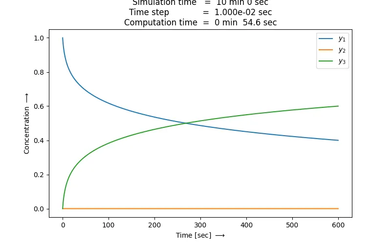
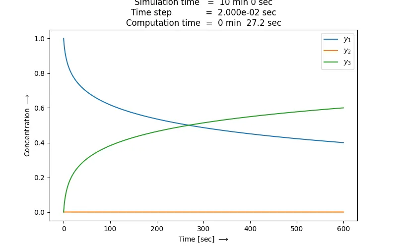
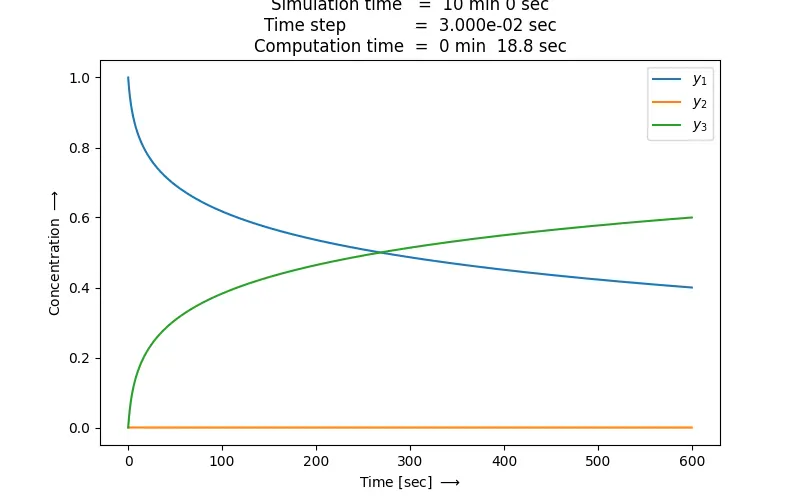
• From the plots, it can be seen that any time step greater than `3e-2` can make the solution unstable so `3e-2` is the ideal time step size.