CHT Analysis on a generic Graphics card

# Abstract:

Conjugate Heat Transfer (CHT) analysis is carried out on a generic graphics card of a computer. Inlet temperature is 300 K & inflow velocity is varied from 1 `m//s` to 5 `m//s`. Steady-state simulations are performed and Heat Transfer Coefficient (HTC) on processor walls is computed in steady-state conditions. Commercially available CFD tool ANSYS® Fluent® 2021 R2 Student version is used.

# Introduction

CHT Analysis

In many applications it is common for fluid flows to interact physically (& sometimes even chemically) with solid surfaces and heat transfer between fluid-solid interface is the most common interaction that can induce changes in temperature, pressure, phase, etc in the fluid with or without the intent of the design.

Hence Conjugate Heat Transfer (CHT) analysis is carried out for graphics card simulations as well which allows for the simulation of heat transfer between solid and fluid domains by exchanging thermal energy at the interfaces between them.

Typical applications of CHT analysis are the simulation of heat exchangers, cooling of electronic equipment, and general-purpose cooling and heating systems.

Graphics card

A graphics card generates a feed of output images to a display device such as a computer monitor. The GPU (Graphics Processing Unit) is the part that processes digital signals & hence generates the highest amount of heat which needs to be dissipated by fins mounted atop it for proper working.

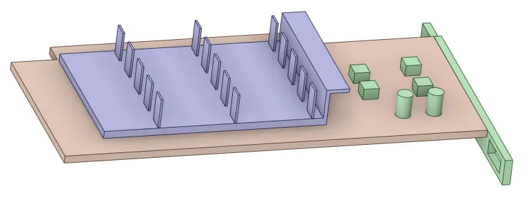
A generic graphics card is shown below. The purple region is the fins, the brown region is the PCB. The capacitors & memory modules are shown in green color.

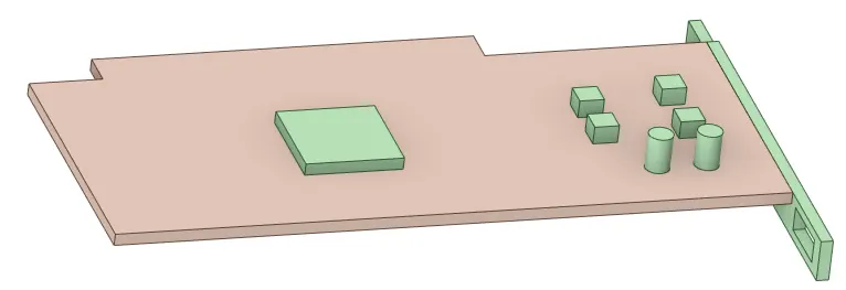
The processor is located between the PCB and fins as shown below.

# Component materials:

Graphics card is made up of many different materials. Their properties are listed below,

Part	Material	Density at 300 K `(kg//m^3)`	Specific heat `(J//(kg K))`	Thermal conductivity `(W//(m K))`
PCB	FR-4	1850	1150	0.294
Processor	Silicon	2329	700	148
Fins	Aluminum	2719	871	202.4

FR-4 and Silicon are created in FLUENT explicitly using `create//edit` materials option as they are not predefined in FLUENT database.

# Numerical model:

Turbulence model

For reduced computational effort RANS based SST `k-omega` turbulence model is used with standard wall functions for near-wall modeling. The `y^+` values are checked after a few initial iterations and also during post-processing so that they fall in the desired range of 1<y^+<10.

Solution method
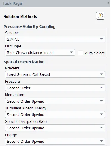
The solution procedure is iterative and is based on SIMPLE scheme for Pressure-Velocity coupling. The discretization is `2^(nd)` order for pressure and `2^(nd)` order upwind for other variables. The gradient is computed using the Least-squares cell-based method. Commercially available CFD tool ANSYS® Fluent® 2021 R2 Student version is used which has a limit of 512,000 cells in the mesh.

# Computational domain:

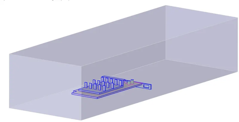
The computational domain is divided into the fluid domain and the solid domain. The common surface of the interface between them is the shared topology so as to allow perfect mesh connectivity across the entire domain. The solid domain is meshed more finely than the fluid domain.

# Boundary Conditions:

# Calculations

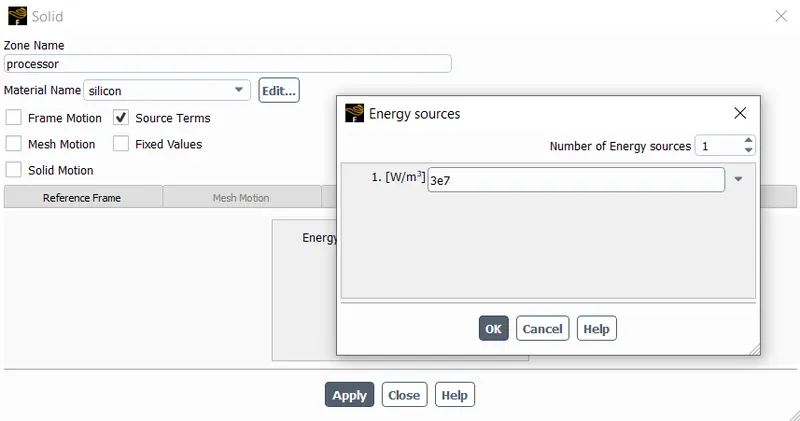
The heat generation in graphics cards varies significantly based on design. For instance, Nvidia’s GTX 1050 has thermal design power (TDP) of 75W. GPU dimensions on a generic graphics card are 50×50 mm thus heat generation in the GPU is,

`H_g = 75/(50"x"50"x"1) = 0.03" "W//mm^3 = 3"x"10^7 W//m^3`

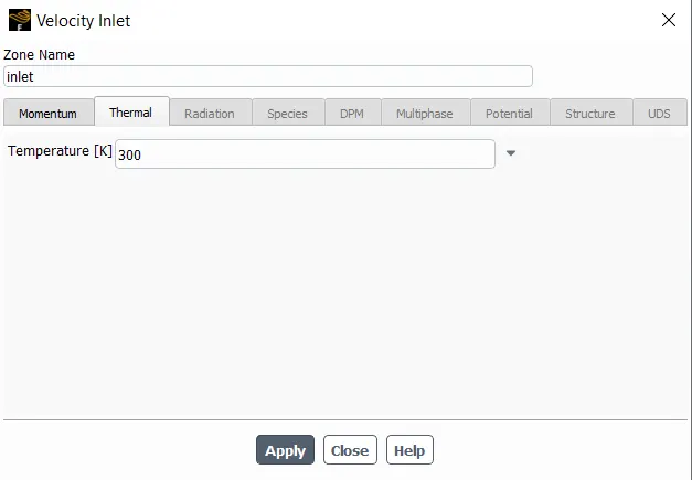
Boundary conditions were set as 'velocity inlet' at inlet faces with velocity normal to surface at 300 K, 'pressure outlet' at outlet face, 'wall' on solid surfaces with no-slip & source term on the processor as 3x10^7 W//m^3.

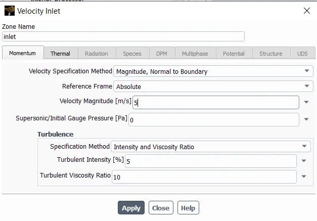
The remaining surfaces were set as ‘wall’ with coupled conditions.

# Solver settings:

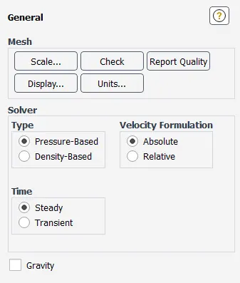
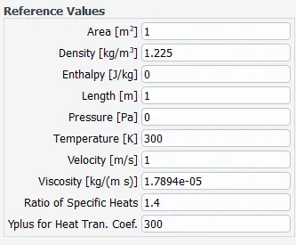
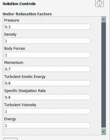
Since the mach no. (`5//sqrt (gamma R T) = 0.01515`) of flow is less than `0.3` pressure based steady-state solver is used for all simulations with pressure-velocity coupling using SIMPLE algorithm. Least squares cell-based method is used for computing gradients

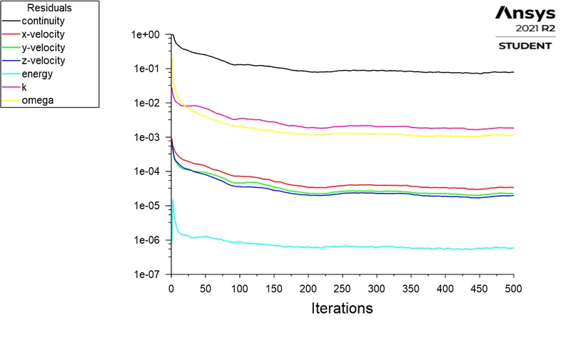
SST `k-omega` turbulence model was selected with `Y^+<10`. Material properties were set accordingly. All simulations were carried out for 500 iterations after hybrid initialization.

# Baseline Simulation:

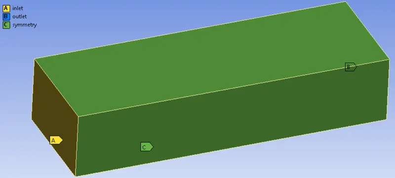
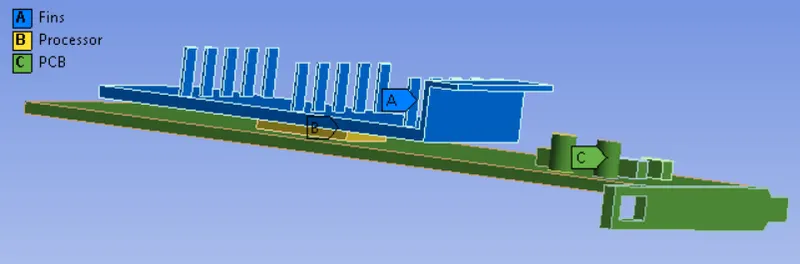
Named selections

Mesh

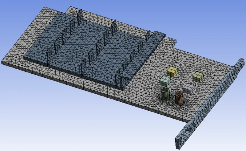
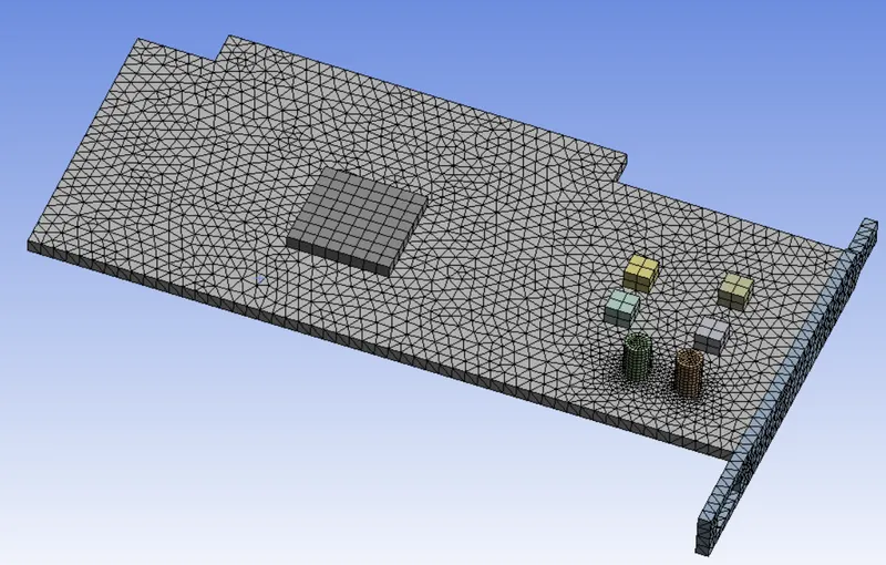
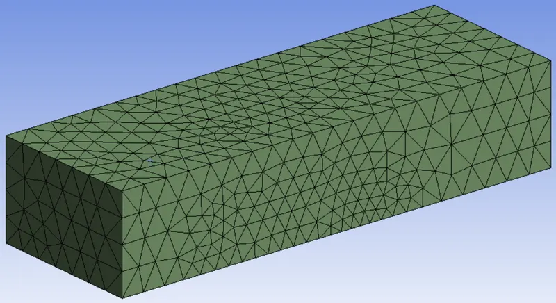
• Baseline simulation was done with an inlet velocity of 5m//s and a coarse mesh shown below.
• The global mesh element size is 10.289 mm and the local element size is as follows,

  Component	Element size for body sizing	Capture curvature
  Fins	1 mm	Yes
  Processor	1 mm	No
  PCB	1 mm	Yes

Convergence plots

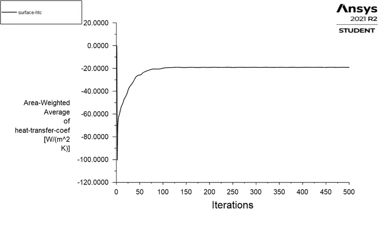
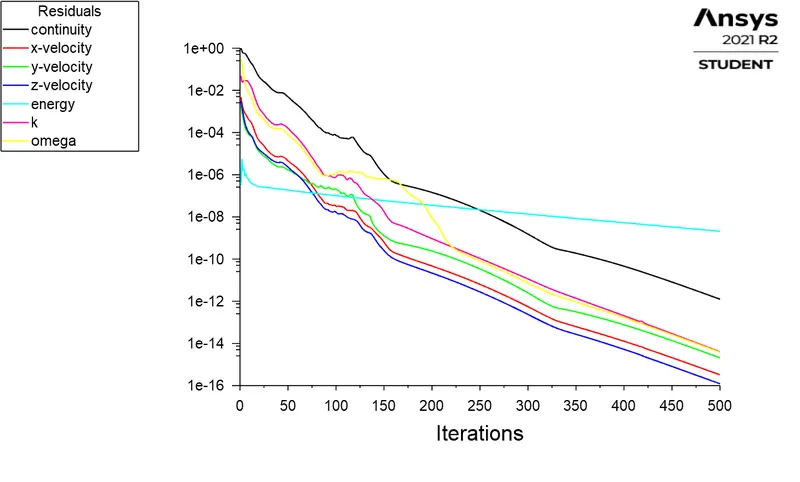
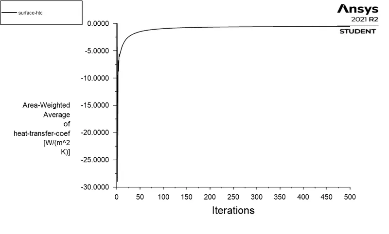
• It can be seen that the solution has converged to a steady-state value since an approximately flat line is visible on HTC and residual plots as shown below.
• A negative HTC value indicates that heat flows from GPU to the cooler surrounding airflow.

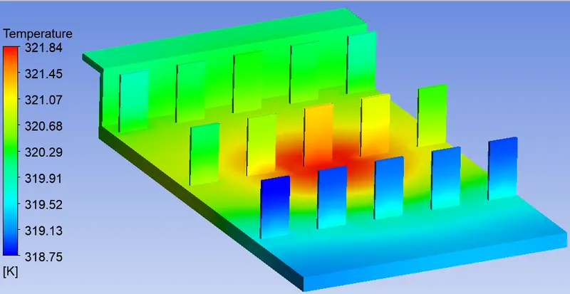
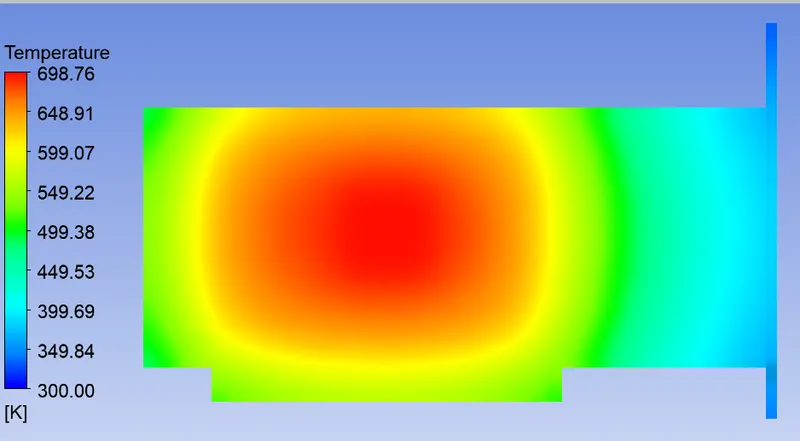
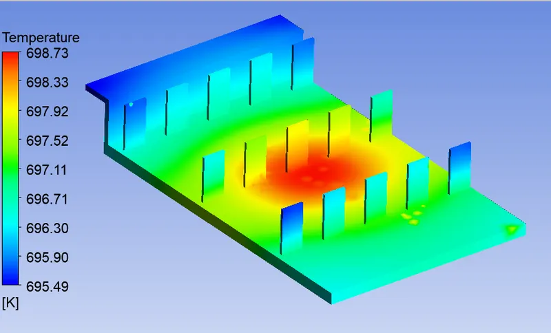
Temperature contours

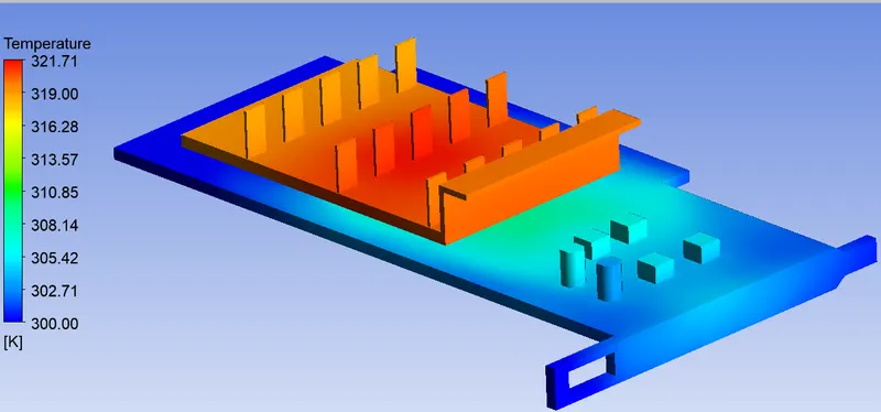
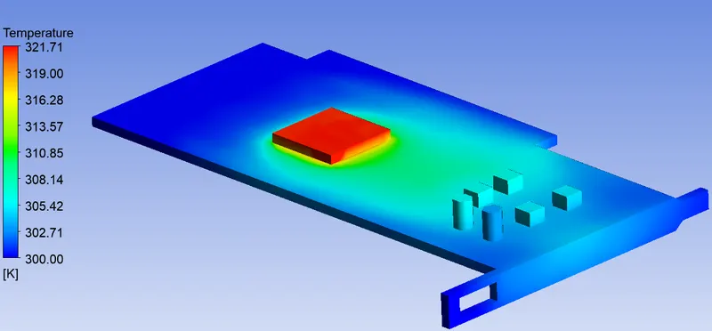
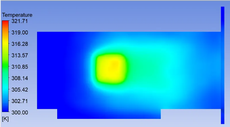
• It can be seen that the temperature on processor walls remains nearly constant (since it is a heat source) and varies over fin surfaces.
• Hot spots are seen in regions surrounding GPU on the PCB board. Temperature is higher in the middle of the fin plate and under PCB where GPU is mounted.
• Temperature is lower at the back end of the fin walls.

# Simulations with refined mesh:

Mesh

• Again the simulation was done with an airflow velocity of 5m/s.
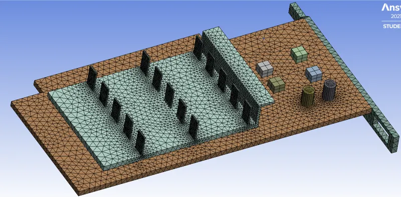
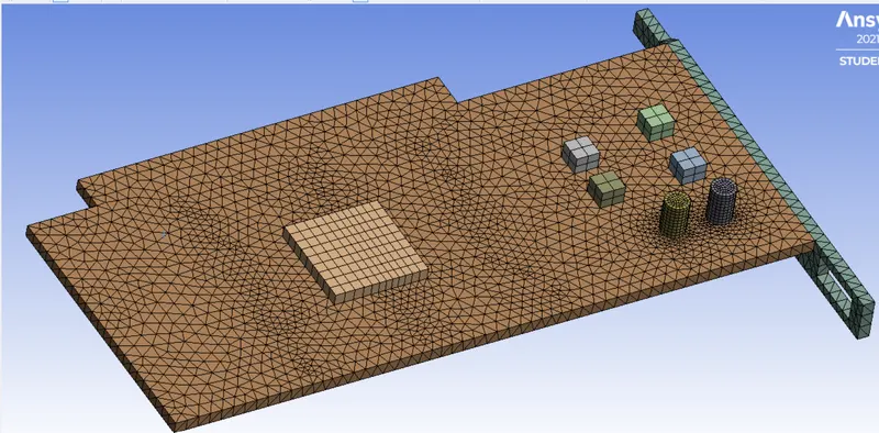
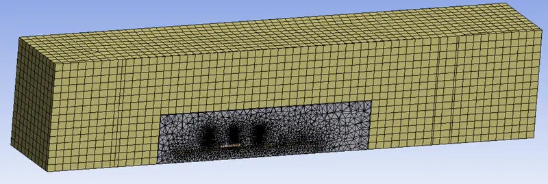
• For effectively capturing flow features and reducing computation load surrounding region near the graphics card is meshed with tetrahedral elements and the outer region where flow variation is less is meshed with hexahedral elements.
• Refinement is also done on the fin surfaces, processor, and PCB board. This is so because the temperature varies significantly in these regions.
• Global mesh settings have multizone option with a global element size of 3 mm and local mesh settings are as follows,

  Component	Element size	Capture curvature
  Fins (face sizing)	0.25 mm	Yes
  Processor (body sizing)	1 mm	Yes
  PCB (body sizing)	1 mm	Yes

Convergence plots

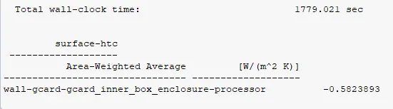
• The solution converges to a much smaller value of HTC through processor walls and also in fewer iterations. This is due to increased accuracy because of finer mesh.

Temperature contours

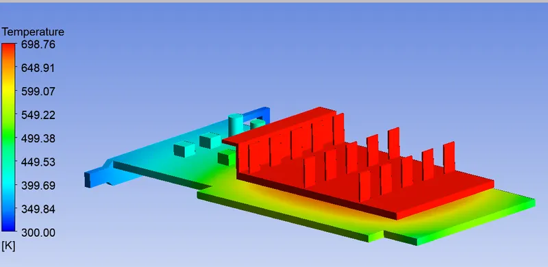
• The temperature contours are similar except for values.
• Also, the temperature is distributed more evenly and spread over a larger area on PCB.

# Conclusion:

• Two more simulations were done at velocities of 3 m/s and 1 m/s with refined mesh. Temperature contours are similar and only the key results are tabulated below.

  Flow velocity `(m//s)`	HTC on GPU `(W//(m^2 K))`	Max. temperature at GPU (K)
  5	0.5824	698
  3	0.5705	706.2
  1	0.5575	717.2

• As expected an increased flow velocity cools GPU more efficiently although the HTC remains nearly the same.
• Hot spots are located directly above and below the GPU and need to be addressed accordingly.
• Fins situated on the inlet side are a bit hotter than fins at the back end. This is due to heat dissipation by convection along fin plate length.