Solving the steady and unsteady 2D heat conduction problem
Transient 2D heat conduction:
Governing equation for transient 2D heat conduction (without heat generation) is,
`(del T)/(del t ) - alpha.((del^2 T)/(del x^2 )+(del^2 T)/(del y^2 ))=0`
We will use Foward differencing for time derivative (for time marching) and `2^(nd)` order Central difference for spatial derivatives (so as to implement jacobi & GS methods).
`(DeltaT_(i,j)^(n+1)-DeltaT_(i,j)^n)/(Deltat) - alpha.((DeltaT_(i-1,j) - 2.DeltaT_(i,j) + DeltaT_(i+1,j))/(Deltax^2) + (DeltaT_(i,j-1) - 2.DeltaT_(i,j) + DeltaT_(i,j+1))/(Deltay^2)) = 0`
`therefore` `(DeltaT_(i,j)^(n+1)-DeltaT_(i,j)^n)/(Deltat) = alpha.((DeltaT_(i-1,j) - 2.DeltaT_(i,j) + DeltaT_(i+1,j))/(Deltax^2) + (DeltaT_(i,j-1) - 2.DeltaT_(i,j) + DeltaT_(i,j+1))/(Deltay^2))`
Where superscript denotes the time level and subscript denotes the grid point. So our numerical stencil is,
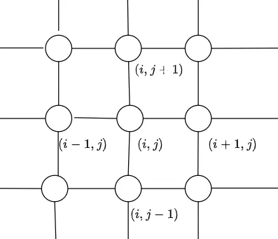
Using notations,
`T_L = " Left grid point"`
`T_R = " Right grid point"`
`T_B = " Bottom grid point"`
`T_T = " Top grid point"`
& `T_P = " Grid point at which the equation is solved at"`
`therefore` `(DeltaT_P^(n+1)-DeltaT_P^n)/(Deltat) = alpha.((DeltaT_L - 2.DeltaT_P + DeltaT_R))/(Deltax^2) +alpha. ((DeltaT_B-2.DeltaT_P + DeltaT_T))/(Deltay^2)`
Rearranging,
`DeltaT_P^(n+1) + DeltaT_P^n = K_1.(DeltaT_L - 2.DeltaT_P + DeltaT_R) + K_2. (DeltaT_B-2.DeltaT_P + DeltaT_T)` where `K_1 =alpha.(Deltat)/(Deltax^2) ` & `K_2 = alpha.(Deltat)/(Deltay^2)`
When the RHS of above equation is evaluated at `n^(th)` time level the equation is called explicit and if it is evaluted at `(n+1)^(th)` time level the equation is called implicit.
Implicit form,
`DeltaT_P^(n+1) = (1/(1+2K_1+2K_2)).(DeltaT_P^n + K_1.(DeltaT_L + DeltaT_R)^(n+1) + K_2. (DeltaT_B + DeltaT_T)^(n+1))`
Explicit form,
`DeltaT_P^(n+1) = DeltaT_P^n .(1-2K_1-2K_2)+ K_1.(DeltaT_L + DeltaT_R)^n + K_2. (DeltaT_B + DeltaT_T)^n`
Steady 2D heat conduction:
In the case of steady-state, the time derivative term is absent so,
`(del^2 T)/(del x^2 )+(del^2 T)/(del y^2 )=0`
Discretizing using the above numerical stencil,
`(DeltaT_L - 2.DeltaT_P + DeltaT_R)/(Delta x^2 ) + (DeltaT_B-2.DeltaT_P + DeltaT_T)/(Delta y^2)=0`
`DeltaT_P ^n=(Delta y^2)/(Delta x^2 +Delta y^2).(DeltaT_L + DeltaT_R)^n + (Delta x^2)/(Delta x^2 +Delta y^2). (DeltaT_B+ DeltaT_T)^n`
`therefore` `DeltaT_P ^n=K_1.(DeltaT_L + DeltaT_R)^n + K_2. (DeltaT_B+ DeltaT_T)^n` where `K_1=(Delta y^2)/(Delta x^2 +Delta y^2)` & `K_2=(Delta x^2)/(Delta x^2 +Delta y^2)`
Due to abscence of time derivative term this equation can only be written in explicit form.
Point iterative Techniques:
Jacobi method: In this method, the value of `T_P^(n+1)` from the previous time step is taken as a guess and then the value from successive iterations in the convergence loop is used to evaluate `T_P^(n+1)`.
Gauss-Siedel method: In this method, the value of `T_P^(n+1)` from the previous time step is taken as a guess and then the value from successive iterations in the convergence loop along with values from the current time step is used to evaluate `T_P^(n+1)`.
SOR(Successive Over Relaxation) method: This method uses the value of `T_P^(n+1)` provided by Jacobi or G-S method and upscales them so that the solution converges faster.
MATLAB Program for 2D transient and steady-state analysis:
- In the main code, we first define inputs for our problem. An array of no. of time steps is initialised so as to simulate the transient state. Immediately after we generate a 40x40 temperature grid along with the boundary conditions.
- The next code block generates user interface and takes inputs using fprintf() & input() functions respectively. These inputs are then validated.
- In the for loop based on user inputs, appropriate if else statements execute a specific solver function. Within if else , tic & toc functions are used to measure the computation time of solvers. The outputs from the solver functions are stored and used to plot temperature distribution for the given no. of time steps in for loop. contourf() plots temperature distribution in the loop and using pause() we obtain a simulation of transient states.
- Lastly, labels and information are added. MAIN CODE
clearvars close all clc % Inputs for 2D heat conduction nt = linspace(100,2000,20); % Array of for different No. of time steps nx = 40; ny = nx; % Square 40x40 space grid L = 1; % Length of square domain = 1 m dx = L/(nx-1); % x space step dy = L/(ny-1); % y space step dt = 0.1; % Time step alpha = 5.55e-4; % Diffusivity % Initial guess value for Temprature grid T = 300*ones(nx,ny); % Setting boundary conditions T(1,:) = 600; T(end,:) = 900; T(:,end) = 800; T(:,1) = 400; T(1,1) = (400+600)/2; % Setting average temprature at corner nodes T(1,end) = (600+800)/2; T(end,end) = (900+800)/2; T(end,1) = (900+400)/2; % BLOCK 1: User interface for selecting 2D heat cond. solver fprintf('Solve 2D heat conduction equation for:'); fprintf('n (1) Transient state (2) Steady staten'); c1 = input(' Your choice: '); if c1==1 fprintf('Select type of equation:'); fprintf('n (1) Implicit (2) Explicitn'); c2 = input(' Your choice: '); else c2 = 2; end fprintf('Select method for solving the equation:'); fprintf('n (1) Jacobi (2) Gauss-Sidiel (3) SOR with GSn'); S_method = input(' Your choice: '); % Checking validity of user inputs if (~ismember(c1,[1 2])||~ismember(c2,[1 2])||~ismember(S_method,[1 2 3])) disp('Undefined input value! Re-run the program and try again'); return else disp(' Executing...'); end % BLOCK 2: solving & plotting x = linspace(0,L,nx); y = linspace(0,L,ny); c_t = 0; % Initialising computation time storing variable figure('Position',[400 50 700 700]); for m = 1:length(nt) if c1==1 if c2==1 tic [T1,iter] = trans_imp_solver(nt(m),ny,nx,dx,dy,dt,alpha,T,S_method); c_t = toc; else tic [T1,iter] = trans_exp_solver(nt(m),ny,nx,dx,dy,dt,alpha,T,S_method); c_t = toc; end else tic [T1,iter] = steady_exp_solver(ny,nx,dx,dy,T,S_method); c_t = toc; end % Plotting results num_iter = iter; [c,h] = contourf(x,y,T1); set(gca,'Ydir','reverse'); xlabel('x axis'); ylabel('y axis'); str1 = "Real time = " + nt(m)*dt + " seconds"; title(str1); if c1==2 break end pause(3/length(nt)) % Adjusting pause duration as per nt hold on end % Labelling plot clabel(c,h,'LabelSpacing',100); str1 = ["implicit" "explicit"]; str2 = [" Jacobi " " Gauss-Seidel " " SOR (with GS) "]; if c1==1 title("2D Temprature variation in Transient states",{"using "+... str1(c2)+str2(S_method)+"method :-","No. of iterations(at 200s) = " + num_iter,... "Computation time(at 200s) = "+c_t+" s",... "Real time = 200 s"}); else title("2D Temprature variation in steady state",{"using explicit"+... str2(S_method)+"method:-","No. of iterations = " + num_iter,... "Computation time(at 200s)= "+c_t+" s"}); end % END OF PROGRAM - The function for solving the transient problems using implicit equation i.e. solving trans_imp_solver() intakes no. of time steps, no. of nodes in x & y, time step, space steps, diffusivity, Temperature grid matrix & S_method; a total of 8 parameters. Then it initialises equation constants and other variables to be used in loops.
- For each iteration of time loop the convergence loop updates the values in T until absolute error becomes less than tolerance limit. switch is used to select the equation to be executed inside space loops. Told is updated for every iteration of convergence loop while T_prev is updated at every iteration of time loop. Solved temp. matrix is returned as output along with no. of iteration in convergence loop for given nt.
- trans_exp_solver() and steady_exp_solver() work in the same fashion except that steady_exp_solver() doesn't intakes nt, dt & alpha. FUNCTION CODES
function [T1,n_iter] = trans_imp_solver(nt,ny,nx,dx,dy,dt,alpha,T,s_method)

tol = 1e-4;    % Error tolerance at convergence
% Defining constants in implicit equations
k1 = alpha*dt/dx^2;
k2 = alpha*dt/dy^2;
term(1) = 1/(1 + 2*k1 + 2*k2);
term(2) = k1*term(1);
term(3) = k2*term(1);
a = 1.1;      % Scaling parameter for SOR method

 % Initialising variables & arrays
 error = 1;
 Told = T;
 T_prev = T;
 iter = 0;

    for n = 1:nt  % Time loop
        while(error > tol) % Convergence loop
            for j = 2:ny-1          % x Space loop
                for i = 2:nx-1      % y space loop
                   switch s_method
                       case 1 % Implicit Jacobi Method
                             T(i,j) = term(1)*T_prev(i,j) +...
                             term(2)*(Told(i-1,j) + Told(i+1,j)) +...
                             term(3)*(Told(i,j+1)+Told(i,j-1));
                       case 2 % Implicit Gauss-Seidel Method
                             T(i,j) = term(1)*T_prev(i,j) +...
                             term(2)*(T(i-1,j) + Told(i+1,j)) +...
                             term(3)*(Told(i,j+1)+T(i,j-1));
                       case 3 % Implicit SOR with GS Method
                             T(i,j) = (1-a)*Told(i,j)+ a*( term(1)*T_prev(i,j) +...
                             term(2)*(T(i-1,j) + Told(i+1,j)) +...
                             term(3)*(Told(i,j+1)+T(i,j-1)) );
                   end
                end
            end
            error = max(max(abs(T-Told))); % Using max two times to find
            Told = T;                      % greatest error value in
            iter = iter+1;                 % (T-Told) matrix
        end
        T_prev = T; % Updating T_prev
        error = 1;  % reseting error
    end
 T1 = T;
 n_iter = iter;
end
function [T1,n_iter] = trans_exp_solver(nt,ny,nx,dx,dy,dt,alpha,T,s_method) tol = 1e-4; % Error tolerance at convergence % Defining constants in explicit equations k1 = alpha*dt/dx^2; k2 = alpha*dt/dy^2; term(1) = (1 - 2*k1 - 2*k2); term(2) = k1; % CFl_x term(3) = k2; % CFL_y a = 1.1; % Scaling parameter for SOR method % Initialising variables & arrays error = 1; Told = T; T_prev = T; iter = 0; for n = 1:nt % Time loop while(error > tol) % Convergence loop for j = 2:ny-1 % Space loops for i = 2:nx-1 switch s_method case 1 % Explicit Jacobi Method T(i,j) = term(1)*T_prev(i,j) +... term(2)*(Told(i-1,j) + Told(i+1,j)) +... term(3)*(Told(i,j+1)+Told(i,j-1)); case 2 % Explicit Gauss-Seidel Method T(i,j) = term(1)*T_prev(i,j) +... term(2)*(T(i-1,j) + Told(i+1,j)) +... term(3)*(Told(i,j+1)+T(i,j-1)); case 3 % Explicit SOR with GS Method T(i,j) = (1-a)*Told(i,j)+ a*( term(1)*T_prev(i,j) +... term(2)*(T(i-1,j) + Told(i+1,j)) +... term(3)*(Told(i,j+1)+T(i,j-1)) ); end end end error = max(max(abs(T-Told))); % Using max two times to find Told = T; % greatest error value in iter = iter+1; % (T-Told) matrix end T_prev = T; error = 1; end T1 = T; n_iter = iter; endfunction [T1,n_iter] = steady_exp_solver(ny,nx,dx,dy,T,s_method) tol = 1e-4; % Error tolerance at convergence % Defining constants in explicit equations k1 = 0.5*dy^2/(dx^2+dy^2); k2 = 0.5*dx^2/(dx^2+dy^2); term(1) = k1; % CFL_y term(2) = k2; % CFl_y a = 1.1; % Scaling parameter for SOR method % Initialising variables & arrays error = 1; Told = T; iter = 0; while(error > tol) % Convergence loop for j = 2:ny-1 % Space loops for i = 2:nx-1 switch s_method case 1 % Explicit Jacobi Method T(i,j) = term(1)*(Told(i-1,j) + Told(i+1,j)) +... term(2)*(Told(i,j+1)+Told(i,j-1)); case 2 % Explicit Gauss-Seidel Method T(i,j) = term(1)*(T(i-1,j) + Told(i+1,j)) +... term(2)*(Told(i,j+1)+T(i,j-1)); case 3 % Explicit SOR with GS Method T(i,j) = (1-a)*Told(i,j)+ a*( ... term(1)*(T(i-1,j) + Told(i+1,j)) +... term(2)*(Told(i,j+1)+T(i,j-1)) ); end end end error = max(max(abs(T-Told))); % Using max two times to find Told = T; % greatest error value in iter = iter+1; % (T-Told) matrix end T1 = T; n_iter = iter; end
Program Outputs:
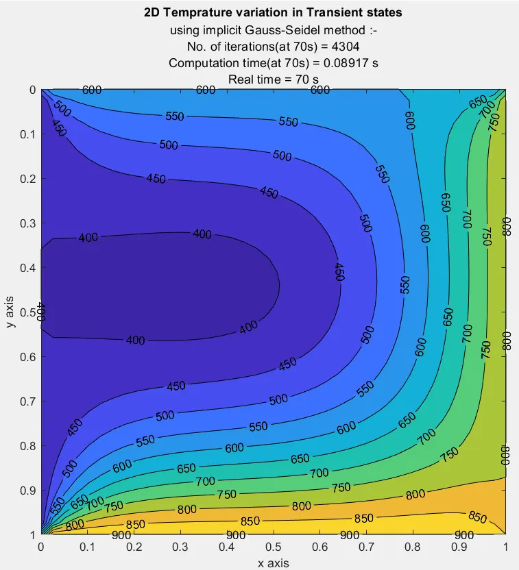
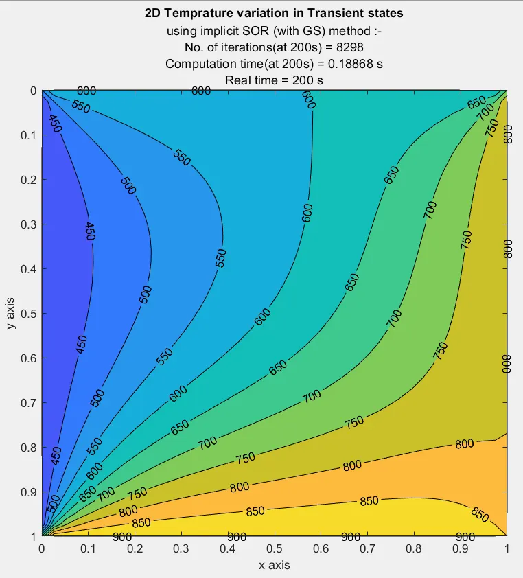
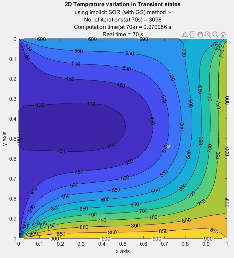
1) Transient 2D heat conduction, using implicit equations.
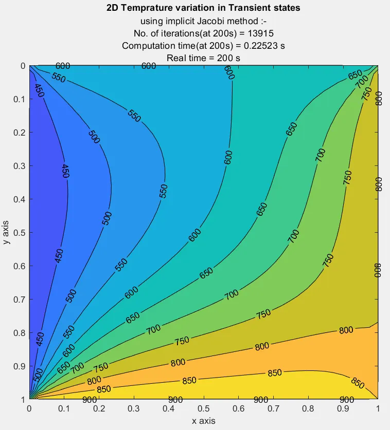
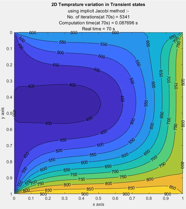
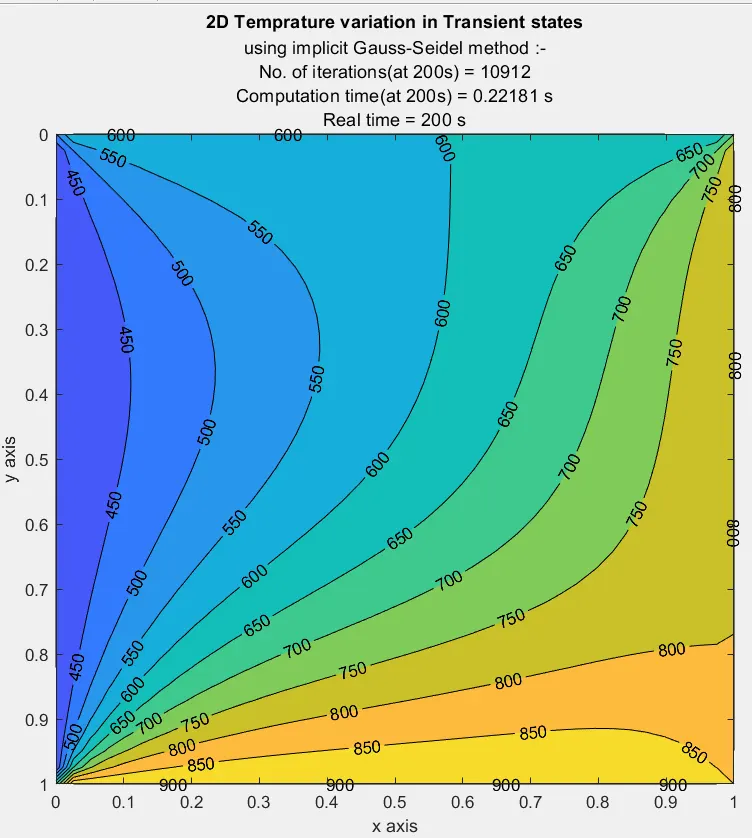
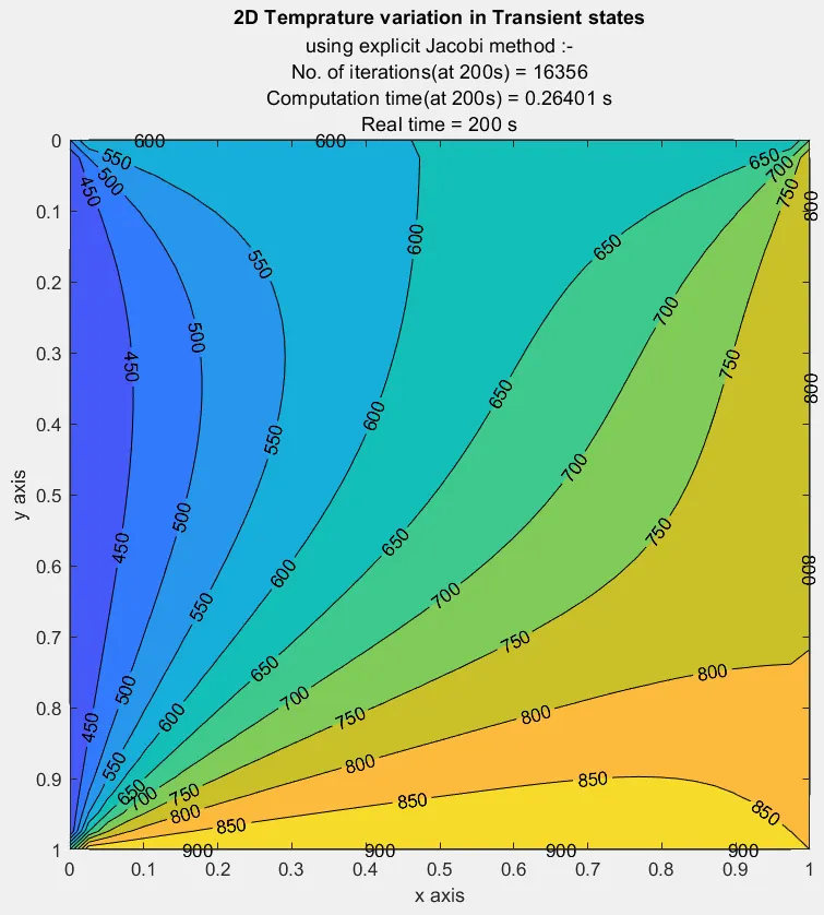
2) Transient 2D heat conduction, using explicit equations.
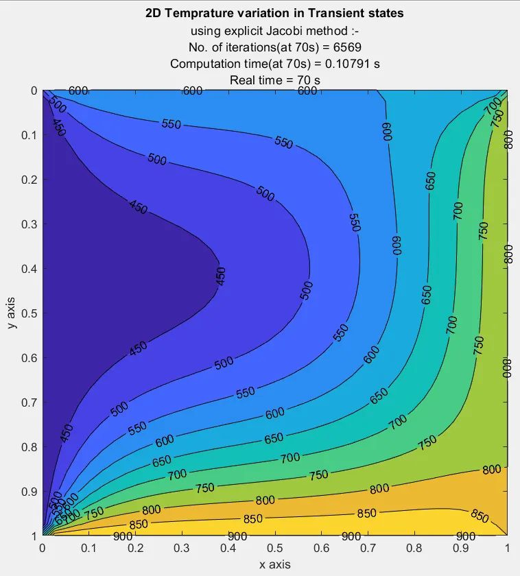
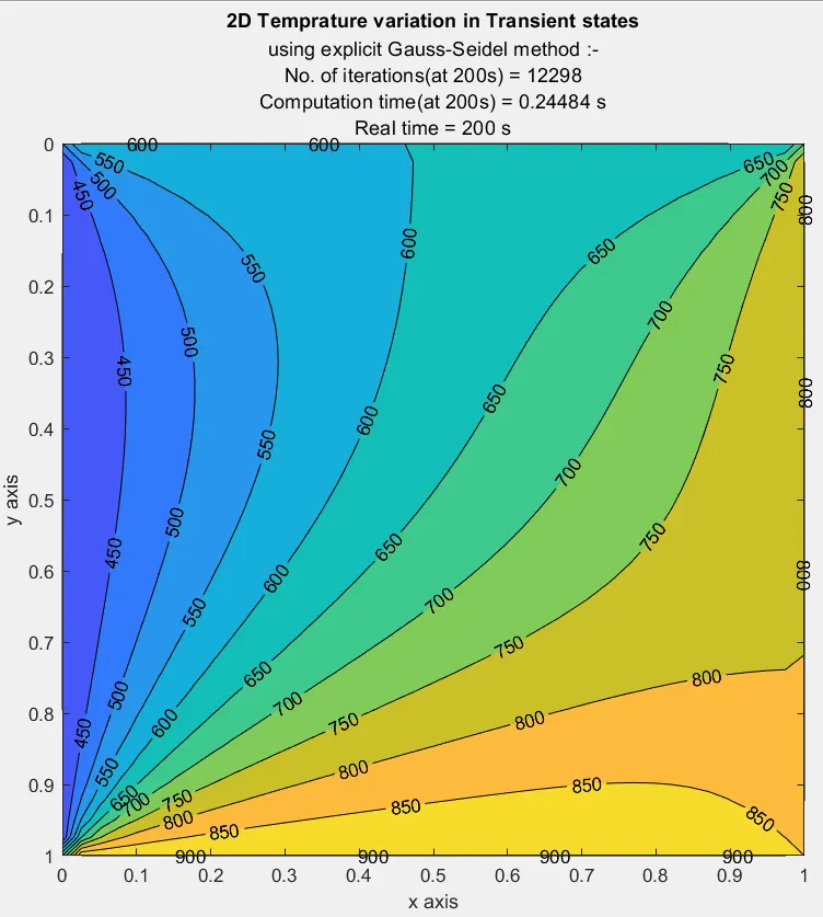
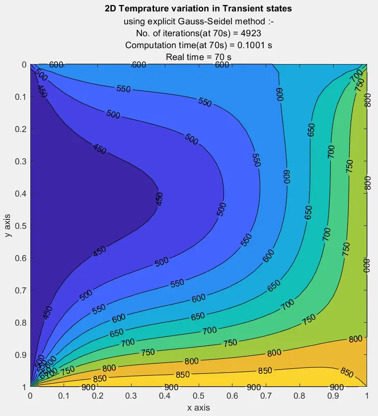
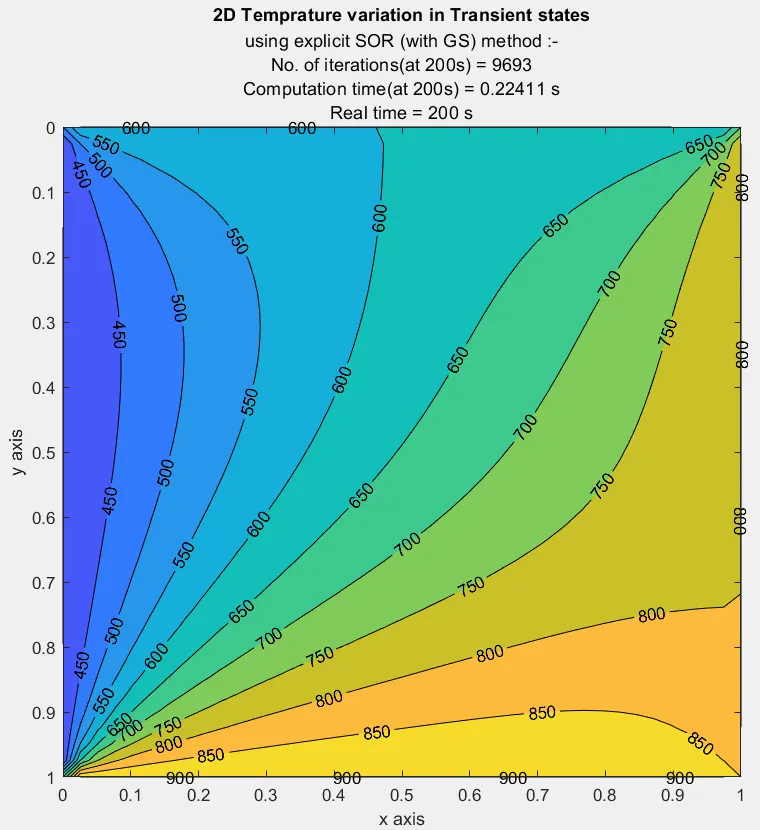
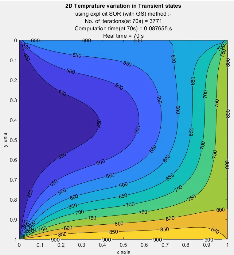
3) Steady 2D heat conduction, using explicit equations.
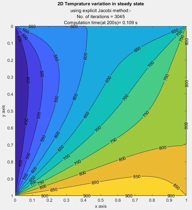
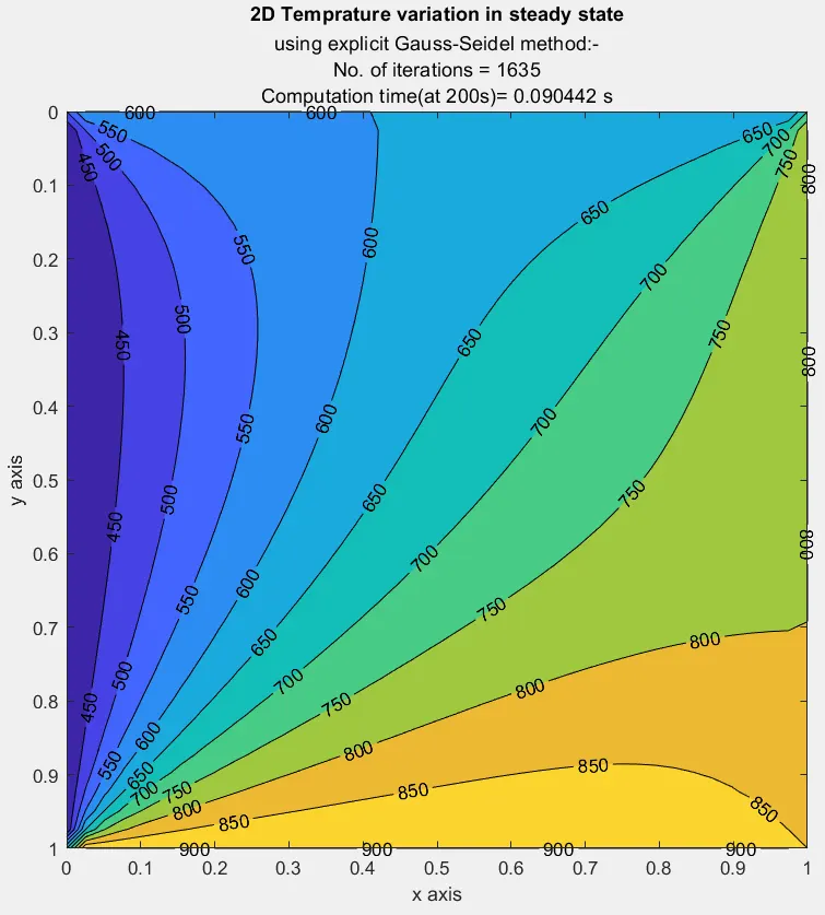
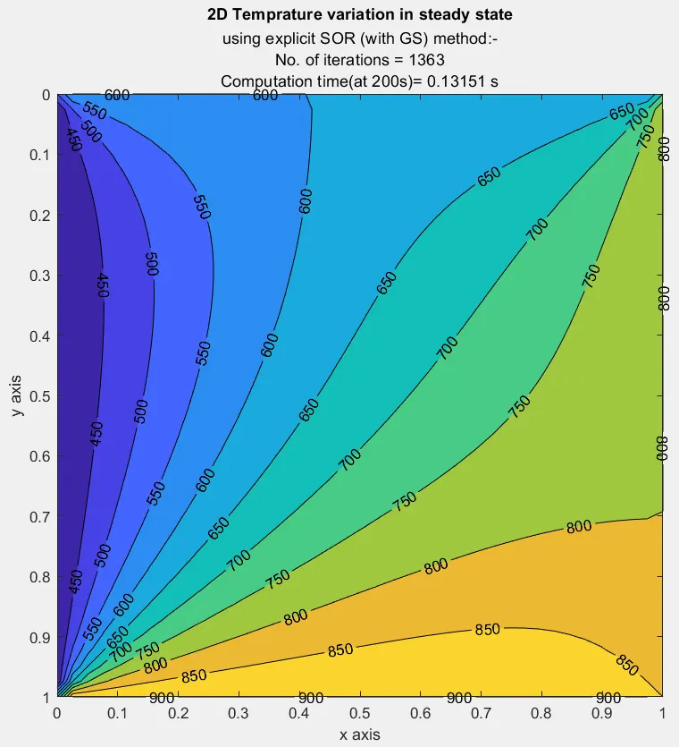
Conclusion:
- The outputs for transient phenomena were similar for the same real times. This shows the reliability of iterative methods.
- But the no. of iterations in the convergence loop differ because the methods converge at different speeds.
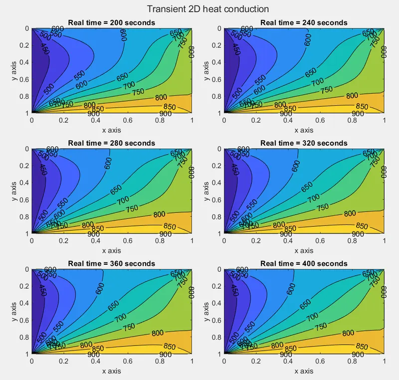
- Again in the steady-state solution, we find similar plots which reapprove the reliability of these methods. However, it is observed that plots of steady-state and transient state at time 200 sec match closely. So it is appropriate to assume that the system reaches a steady-state after 200 seconds. This can be confirmed by solving beyond 200 sec and observing very little change as shown below.
- The program output can be summarised as,
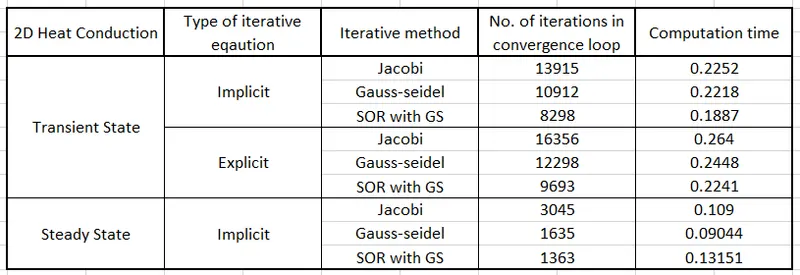
So it can be concluded that Computation time decreases as Jacobi>Gauss-seidel>SOR.