Adiabatic Flame Temperature calculation
# Aim:
For this project, we are going to compute & plot Adiabatic flame temperature (AFT) during the combustion of methane (natural gas) using python and Cantera package. Our main objectives are:
- Find AFT variation with Equivalence ratio in a constant volume chamber and compare results with and without using cantera package.
- Flame temperature variation with Heat loss in a constant pressure chamber.
- AFT variation with respect to Alkane, Alkene & Alkyne (2 C-atom variants only).
- AFT variation with respect to the number of carbon atoms in the hydrocarbon chain of alkane.
# Introduction:
AFT
The adiabatic flame temperature is the maximum temperature that can be achieved during a combustion reaction provided there is no heat loss to the surroundings i.e. adiabatic condition. Depending on the process are two types of AFTs constant pressure and constant volume. Constant volume AFT is always higher than constant pressure AFT as it occurs without any work transfer by combusting mixture.
LHV
The lower heating value (LHV; net calorific value; NCV, or lower calorific value; LCV) is a measure of available thermal energy produced by the combustion of fuel. The LHV is determined by bringing all the products of combustion back to the original pre-combustion temperature (usually STP) assuming any vapor produced is not condensed.
NASA polynomial
The NASA polynomials have the form:
`(C_p)/R = a_1 + a_2 T + a_3 T^2 + a_4 T^3 + a_5 T^4`
`H/(barRT) = a_1 + a_2 T /2 + a_3 T^2 /3 + a_4 T^3 /4 + a_5 T^4 /5 + a_6/T`
`S/barR = a_1 lnT + a_2 T + a_3 T^2 /2 + a_4 T^3 /3 + a_5 T^4 /4 + a_7`
where `a_1, a_2, a_3, a_4, a_5, a_6` and `a_7` are the numerical coefficients supplied in NASA thermodynamic files.
GRI-mech
To get numerical coefficients we will refer to the thermodynamic file provided by GRI-Mech for the combustion of natural gas. GRI-mech is essentially a list of elementary chemical reactions and associated rate constant expressions. Most of the reactions listed in files by GRI-mech have been studied one way or another in the laboratory and have more or less direct measurements behind them.
Cantera package uses this thermodynamic data file to predict natural gas combustion. We will also use the same file but only a few species will be considered.
Practical applications
Fuels provide most energy during combustion under stoichiometric conditions. But this can cause flame temperatures to exceed temperature limits set by the materials in a combustion system. To avoid this the flame temperature is often reduced by adding excess air just enough for safe combustion temperatures.
Inaccurate prediction of AFT for the combustion application can reduce product life or even failure in the worst case.
# Theory:
For each code, we will be using NASA polynomial for evaluating the enthalpy of formation at a given temperature,
`H/(barRT) = a_1 + a_2 T /2 + a_3 T^2 /3 + a_4 T^3 /4 + a_5 T^4 /5 + a_6/T`....`(1)`
Once we have enthalpy we can calculate adiabatic flame temperature by solving an equation in temperature using the Newton-Raphson method.
The first seven coefficients in thermodynamic files are high temperature `(T>=1000 K)` coefficients and the last 7 are low-temperature coefficients `(200 K<T<1000 K)`. The same order is maintained in input arrays storing coefficients.
For constant volume process
`Delta Q = Delta U - P Delta V ("from 1st law")`
`Delta H = Delta U + P Delta V + V Delta P`
`therefore Delta H = (P_fV_f - P_i V_i) (because P Delta V = 0, Delta U = 0)`
`therefore Delta H = barRN_("products"')T_(ad) - barRN_("reactants")T_i`
`therefore (H_("reactants") - H_("products")) - barR( N_("reactants")T_i - N_("products")T_(ad)) = f(T) = 0`. . . `(2)`
For heat loss in constant pressure process
`Delta Q = Delta U - P Delta V ("from 1st law")`
`Delta H = Delta U + P Delta V + V Delta P`
`Delta H = Delta Q `
`therefore (H_("reactants") - H_("products")) - "heat loss factor"*LHV = f(T) = 0`. . .`(3)`
For constant pressure process
Following the derivation above,
`Delta U = - P Delta V`
`Delta H = Delta U + P Delta V + V Delta P`
`Delta H = 0 (because V Delta P = 0)`
`therefore (H_("reactants") - H_("products")) = f(T) = 0`. . .`(4)`
# Coding approach:
PART I
- We will first import the following python packages into our workspace,
- numpy: For faster & efficient array manipulations.
- maplotlib.pyplot: For plotting datasets.
- cantera : chemical kinetics package used for solving chemically reacting laminar flows.
- Next NASA polynomial coefficients from 'gri30' file (for methane) are fed into respective numpy arrays.
- An enthalpy function "h(T)" is defined which takes the coefficient array & given temperature and returns the enthalpy of formation for the species using equation (1).
- Now for constant volume combustion, we need to solve eq. (2) using Newton-Raphson method. Equ. (2) is represented by function "f(T,phi)" which takes Temperature & equivalence ratio as arguments, finds enthalpies for each species, and then selects appropriate reaction based on the value of "phi'" to compute enthalpies of reactants and products.
- A numerical derivative of function "f(T, phi)" is calculated using a first-order forward derivative with step size 1e-6. The function is named "fprime".
- In the main code, we iterate over values of "phi" from 0.05 to 3.0 and apply while loop to implement NR method.
- The guessed adiabatic flame temperature for each value of "phi" is assumed as 1500 K since the flame is expected to be in the high-temperature range. This is why in function "f(T, phi)" we have used high-temperature coefficients for calculating the enthalpy of products.
- The AFT is stored in an array for both techniques, the NR method and the Cantera package. The results are plotted in a single figure for comparison.
import numpy as np
import matplotlib.pyplot as plt
import cantera as ct

# NASA polynomial coefficients from thermodynamic file
# First seven values are high temperature coefficients and rest are low temperature coefficients

CH4_coeff = np.array([7.48514950E-02, 1.33909467E-02, -5.73285809E-06, 1.22292535E-09, -1.01815230E-13, -9.46834459E+03, 1.84373180E+01,
5.14987613E+00, -1.36709788E-02, 4.91800599E-05,-4.84743026E-08, 1.66693956E-11, -1.02466476E+04, -4.64130376E+00])

O2_coeff  = np.array([3.28253784E+00, 1.48308754E-03, -7.57966669E-07, 2.09470555E-10, -2.16717794E-14,-1.08845772E+03, 5.45323129E+00,
3.78245636E+00, -2.99673416E-03, 9.84730201E-06,-9.68129509E-09, 3.24372837E-12, -1.06394356E+03, 3.65767573E+00])

N2_coeff  = np.array([0.02926640E+02, 0.14879768E-02, -0.05684760E-05, 0.10097038E-09, -0.06753351E-13, -0.09227977E+04, 0.05980528E+02,
0.03298677E+02, 0.14082404E-02, -0.03963222E-04, 0.05641515E-07, -0.02444854E-10, -0.10208999E+04, 0.03950372E+02])

CO_coeff  = np.array([2.71518561E+00, 2.06252743E-03, -9.98825771E-07, 2.30053008E-10, -2.03647716E-14, -1.41518724E+04, 7.81868772E+00,
3.57953347E+00, -6.10353680E-04, 1.01681433E-06, 9.07005884E-10, -9.04424499E-13, -1.43440860E+04, 3.50840928E+00])

CO2_coeff = np.array([3.85746029E+00, 4.41437026E-03, -2.21481404E-06, 5.23490188E-10, -4.72084164E-14, -4.87591660E+04, 2.27163806E+00,
2.35677352E+00, 8.98459677E-03, -7.12356269E-06, 2.45919022E-09, -1.43699548E-13, -4.83719697E+04, 9.90105222E+00])

H2O_coeff = np.array([3.03399249E+00, 2.17691804E-03, -1.64072518E-07, -9.70419870E-11, 1.68200992E-14, -3.00042971E+04, 4.96677010E+00,
4.19864056E+00, -2.03643410E-03, 6.52040211E-06, -5.48797062E-09, 1.77197817E-12, -3.02937267E+04, -8.49032208E-01])

# Enthalpy of formation, H(T)
# Takes coefficient array & temperature and returns Enthalpy of formation
def h(c,T):
    R = 8.314 #J/mol K
    return (c[0] + c[1]*T/2 + c[2]*(T**2)/3 + c[3]*(T**3)/4 + c[4]*(T**4)/5 + c[5]/T)*R*T

# Adiabatic flame temperature variation with Equivalence ratio (In constant volume-chamber)
# Lean combustion follows:           CH_4 + (2/phi)(O_2 + 3.76N_2) -->CO_2 + 2H_2O + 7.52(phi)N_2 + 2/(phi - 2)O_2
# Stoichiometric combustion follows: CH_4 + 2(O_2 + 3.76N_2) -->CO_2 + 2H_2O + 7.52N_2
# Rich combustion follows:           CH_4 + (2/phi)(O_2 + 3.76N_2) --> (4/phi - 3)CO_2 + 2H_2O + 7.52(phi)N_2 + (4 - 4/phi)CO
# Function whoose roots are needed, f(T)
def f(T,phi):
    T_STP     = 298.15
    R         = 8.314  #J/mol K

    # Enthalphy of fromation of reactants
    h_CH4_r = h(CH4_coeff[7:-1], T_STP)
    h_O2_r  = h(O2_coeff[7:-1], T_STP)
    h_N2_r  = h(N2_coeff[7:-1], T_STP)

    H_r     = h_CH4_r + (2/phi)*(h_O2_r + 3.76*h_N2_r)
    N_r     = 1 + 2/phi + (2/phi)*3.76

    # Enthaply of formation of products
    h_CO_p  = h(CO_coeff[0:6], T)
    h_CO2_p = h(CO2_coeff[0:6], T)
    h_H2O_p = h(H2O_coeff[0:6], T)
    h_N2_p  = h(N2_coeff[0:6], T)
    h_O2_p  = h(O2_coeff[0:6], T)

    if phi < 1:
        H_p     =  h_CO2_p + 2*h_H2O_p + (7.52/phi)*h_N2_p + (2/phi - 2)*h_O2_p
        N_p     =  1 + 2 + 7.52/phi + 2/phi - 2
    elif phi == 1:
        H_p     =  h_CO2_p + 2*h_H2O_p + 7.52*h_N2_p
        N_p     =  1 + 2 + 7.52
    else:
        H_p     = (4/phi - 3)*h_CO2_p + 2*h_H2O_p + (7.52/phi)*h_N2_p + (4 - 4/phi)*h_CO_p
        N_p     =  4/phi - 3 + 2 + 7.52/phi + 4 - 4/phi

    return    (H_r - H_p) - (N_r*R*T_STP - N_p*R*T)

# Numerical derivative of f(T), f'(T)
# Finds first order forward derivative of f(T) function for step size 1e-6
def fprime(T, phi):
    return (f(T + 1e-6, phi) - f(T, phi))/1e-6

# Using simple 1 step reaction mechanism (no intermidiatory species)
T_g       = 1500    # Kelvin
tol       = 1e-3
alpha     = 0.5                      # Under-relaxation factor
AFT_p     = np.array([])             # Initializing array

phi_range = np.linspace(0.05,3,60)   # Phi varies from 0.05 to 3

for phi in phi_range:
    T_guess = T_g                    # Resetting guesss value

    # Newton-Raphson approximation
    while( abs(f(T_guess,phi)) > tol):
        T_guess = T_guess - alpha*( f(T_guess,phi)/fprime(T_guess, phi) )

    AFT_p = np.append(AFT_p,T_guess)  # Appends values to array

# Using Cantera package
gas = ct.Solution('gri30.xml')
AFT_c = np.array([])                 # Initializing array

for phi in phi_range:
    gas.TPX = 289.15,101325,{'CH4':1, 'O2':2/phi, 'N2':7.52/phi}
    gas.equilibrate('UV','auto')
    AFT_c = np.append(AFT_c, gas.T)

# Plotting results
plt.plot(phi_range, AFT_p, '.-r', label = 'Using simple reaction mechanism')
plt.plot(phi_range, AFT_c, '.-g', label = 'Using Cantera')
plt.xlabel(r'Equivalance ratio $(Phi)rightarrow$')
plt.ylabel(r'Adiabatic flame temperature  [K] $rightarrow$')
plt.title(r'AFT vs Equivalence ratio $(phi)$')
plt.xticks(np.arange(0,3 + 0.2,0.2))
plt.yticks(np.arange(500,3000,200))
plt.grid('on')
plt.legend()
plt.show()

# -----------------------------------------------END ----------------------------------------------
-------------------------------------------------------------------------------------------------------------------------------------------------------------------
PART II
- The code for this part is very similar to part I except that we will use equ.(3) as the function to be evaluated by Newton-Raphson.
- Also, cantera package will not be used here as we are only interested in the trend line i.e the effect on AFT, and not the exact values.
- AFT will be calculated at the stoichiometric equivalence ratio here.
import numpy as np
import matplotlib.pyplot as plt

# NASA polynomial coefficients from thermodynamic file,
# First seven values are high temperature coefficients and rest are low temperature coefficients

CH4_coeff = np.array([7.48514950E-02, 1.33909467E-02, -5.73285809E-06, 1.22292535E-09, -1.01815230E-13, -9.46834459E+03, 1.84373180E+01,
5.14987613E+00, -1.36709788E-02, 4.91800599E-05,-4.84743026E-08, 1.66693956E-11, -1.02466476E+04, -4.64130376E+00])

O2_coeff  = np.array([3.28253784E+00, 1.48308754E-03, -7.57966669E-07, 2.09470555E-10, -2.16717794E-14,-1.08845772E+03, 5.45323129E+00,
3.78245636E+00, -2.99673416E-03, 9.84730201E-06,-9.68129509E-09, 3.24372837E-12, -1.06394356E+03, 3.65767573E+00])

N2_coeff  = np.array([0.02926640E+02, 0.14879768E-02, -0.05684760E-05, 0.10097038E-09, -0.06753351E-13, -0.09227977E+04, 0.05980528E+02,
0.03298677E+02, 0.14082404E-02, -0.03963222E-04, 0.05641515E-07, -0.02444854E-10, -0.10208999E+04, 0.03950372E+02])

CO_coeff  = np.array([2.71518561E+00, 2.06252743E-03, -9.98825771E-07, 2.30053008E-10, -2.03647716E-14, -1.41518724E+04, 7.81868772E+00,
3.57953347E+00, -6.10353680E-04, 1.01681433E-06, 9.07005884E-10, -9.04424499E-13, -1.43440860E+04, 3.50840928E+00])

CO2_coeff = np.array([3.85746029E+00, 4.41437026E-03, -2.21481404E-06, 5.23490188E-10, -4.72084164E-14, -4.87591660E+04, 2.27163806E+00,
2.35677352E+00, 8.98459677E-03, -7.12356269E-06, 2.45919022E-09, -1.43699548E-13, -4.83719697E+04, 9.90105222E+00])

H2O_coeff = np.array([3.03399249E+00, 2.17691804E-03, -1.64072518E-07, -9.70419870E-11, 1.68200992E-14, -3.00042971E+04, 4.96677010E+00,
4.19864056E+00, -2.03643410E-03, 6.52040211E-06, -5.48797062E-09, 1.77197817E-12, -3.02937267E+04, -8.49032208E-01])

# Enthalpy of formation, H(T):
# Takes coefficient array & temperature and returns Enthalpy of formation
def h(c,T):
    R = 8.314 #J/mol K
    return (c[0] + c[1]*T/2 + c[2]*(T**2)/3 + c[3]*(T**3)/4 + c[4]*(T**4)/5 + c[5]/T)*R*T

# Flame temperature variation with heat loss (In constant pressure chamber)} }$
# Stoichiometric combustion follows: $CH_4 + 2(O_2+3.76N_2) -->CO_2 + 2H_2O + 7.52N_2$
def f(T,q_loss_factor):
    T_STP     = 298.15

    # Enthalphy of fromation of reactants
    # Uses low temp. coeff. 200 K < T < 1000 K
    h_CH4_r = h(CH4_coeff[7:-1], T_STP)
    h_O2_r  = h(O2_coeff[7:-1], T_STP)
    h_N2_r  = h(N2_coeff[7:-1], T_STP)

    H_r    = h_CH4_r + 2*(h_O2_r + 3.76*h_N2_r)

    # Enthaply of formation of products
    # Uses high temp. coeff. 1000 K < T < 3500 K
    h_CO2_p = h(CO2_coeff[0:6], T)
    h_H2O_p = h(H2O_coeff[0:6], T)
    h_N2_p  = h(N2_coeff[0:6], T)

    H_p     =  h_CO2_p + 2*h_H2O_p + 7.52*h_N2_p

    # Uses low temp. coeff 200 K < T < 1000 K for computing LHV (Lower Heating Value)
    h_CO2_pl = h(CO2_coeff[7:-1], T_STP)
    h_H2O_pl = h(H2O_coeff[7:-1], T_STP)
    h_N2_pl  = h(N2_coeff[7:-1], T_STP)
    H_p_l     = h_CO2_pl + 2*h_H2O_pl + 7.52*h_N2_pl
    LHV      = H_r - H_p_l

    return   (H_r - H_p) - q_loss_factor*LHV

##### $text{Numerical derivative of f(T) at T, } f'(T):-$
# Finds first order forward derivative of f(T) function for step size 1e-6
def fprime(T, q_l_f):
    return (f(T + 1e-6, q_l_f) - f(T, q_l_f))/1e-6

# Using simple 1 step reaction mechanism (no intermidiatory species)
T_g           = 1500    # Kelvin
tol           = 1e-3
alpha         = 0.5                     # Under-relaxation factor
AFT         = np.array([])              # Initializing array
q_loss_factor = np.linspace(0.05,1,51)  # Varying heat loss factor

for q_l_f in q_loss_factor:
    T_guess = T_g                       # Updating guesss value

    # Newton-Raphson approximation
    while( abs(f(T_guess, q_l_f)) > tol):
        T_guess = T_guess - alpha*( f(T_guess, q_l_f)/fprime(T_guess,  q_l_f) )

    AFT = np.append(AFT,T_guess)  # Appends values to array

# Plotting results
plt.plot(q_loss_factor, AFT, '.-b')
plt.xlabel('Heat loss factor $ longrightarrow$')
plt.ylabel('Flame temperature  [K] $ longrightarrow$')
plt.title('Flame temperature vs Heat loss factor')
plt.xticks(np.arange(0,1 + 0.01,0.1))
plt.yticks(np.arange(200,2400,150))
plt.grid('on')
plt.show()

# -----------------------------------------------END ----------------------------------------------
-------------------------------------------------------------------------------------------------------------------------------------------------------------------
PART III
- Again in this part, we are only interested in the trend of AFT for alkane, alkene & alkyne. Hence cantera is not used here as well.
- The function to be evaluated here will be equ.(4) and reactions will be stoichiometric.
- The fuels will be indexed by the variable "fuel" and the corresponding equation will be used to find enthalpy inside function "f(T, fuel)". the remaining code is the same as in part II except that a bar plot will be utilized here.
import numpy as np
import matplotlib.pyplot as plt

# NASA polynomial coefficients from thermodynamic file,
# First seven values are high temperature coefficients and rest are low temperature coefficients

C2H6_coeff = np.array([1.07188150E+00, 2.16852677E-02, -1.00256067E-05, 2.21412001E-09, -1.90002890E-13, -1.14263932E+04, 1.51156107E+01,
4.29142492E+00-5,.50154270E-03, 5.99438288E-05, -7.08466285E-08, 2.68685771E-11, -1.15222055E+04, 2.66682316E+00])

C2H4_coeff = np.array([2.03611116E+00, 1.46454151E-02, -6.71077915E-06, 1.47222923E-09, -1.25706061E-13, 4.93988614E+03, 1.03053693E+01,
3.95920148E+00, -7.57052247E-03, 5.70990292E-05, -6.91588753E-08, 2.69884373E-11, 5.08977593E+03, 4.09733096E+00])

C2H2_coeff = np.array([4.14756964E+00, 5.96166664E-03, -2.37294852E-06, 4.67412171E-10, -3.61235213E-14, 2.59359992E+04, -1.23028121E+00,
8.08681094E-01, 2.33615629E-02, -3.55171815E-05, 2.80152437E-08, -8.50072974E-12, 2.64289807E+04, 1.39397051E+01])

O2_coeff  = np.array([3.28253784E+00, 1.48308754E-03, -7.57966669E-07, 2.09470555E-10, -2.16717794E-14,-1.08845772E+03, 5.45323129E+00,
3.78245636E+00, -2.99673416E-03, 9.84730201E-06,-9.68129509E-09, 3.24372837E-12, -1.06394356E+03, 3.65767573E+00])

N2_coeff  = np.array([0.02926640E+02, 0.14879768E-02, -0.05684760E-05, 0.10097038E-09, -0.06753351E-13, -0.09227977E+04, 0.05980528E+02,
0.03298677E+02, 0.14082404E-02, -0.03963222E-04, 0.05641515E-07, -0.02444854E-10, -0.10208999E+04, 0.03950372E+02])

CO_coeff  = np.array([2.71518561E+00, 2.06252743E-03, -9.98825771E-07, 2.30053008E-10, -2.03647716E-14, -1.41518724E+04, 7.81868772E+00,
3.57953347E+00, -6.10353680E-04, 1.01681433E-06, 9.07005884E-10, -9.04424499E-13, -1.43440860E+04, 3.50840928E+00])

CO2_coeff = np.array([3.85746029E+00, 4.41437026E-03, -2.21481404E-06, 5.23490188E-10, -4.72084164E-14, -4.87591660E+04, 2.27163806E+00,
2.35677352E+00, 8.98459677E-03, -7.12356269E-06, 2.45919022E-09, -1.43699548E-13, -4.83719697E+04, 9.90105222E+00])

H2O_coeff = np.array([3.03399249E+00, 2.17691804E-03, -1.64072518E-07, -9.70419870E-11, 1.68200992E-14, -3.00042971E+04, 4.96677010E+00,
4.19864056E+00, -2.03643410E-03, 6.52040211E-06, -5.48797062E-09, 1.77197817E-12, -3.02937267E+04, -8.49032208E-01])

# Enthalpy of formation, }H(T):-$
# Takes coefficient array & temperature and returns Enthalpy of formation
def h(c,T):
    R = 8.314 #J/mol K
    return (c[0] + c[1]*T/2 + c[2]*(T**2)/3 + c[3]*(T**3)/4 + c[4]*(T**4)/5 + c[5]/T)*R*T

# Adiabatic flame temperature variation in Alkane, Alkenes & Alkyenes (In constant volume-chamber),
# stoichiometric combustion for,
# Alkanes: C_nH_{2n+2} + (3n+1)/2 (O_2+3.76N_2) -->CO_2 + (n+1)H_2O + (3n+1)/2 3.76N_2
# Alkenes: C_nH_{2n+2} + (3n/2) (O_2+3.76N_2) -->CO_2 + nH_2O + (3n/2) 3.76N_2
# Alkynes: C_nH_{2n+2} + (3n-1)/2 (O_2+3.76N_2) -->CO_2 + (n-1)H_2O + (3n-1)/2 3.76N_2
# Function whoose roots are needed, f(T):-
def f(T,fuel):
    T_STP     = 298.15
    R         = 8.314  #J/mol K

    # Enthalphy of fromation of reactants
    h_C2H6_r = h(C2H6_coeff[7:-1], T_STP)
    h_C2H4_r = h(C2H4_coeff[7:-1], T_STP)
    h_C2H2_r = h(C2H2_coeff[7:-1], T_STP)
    h_O2_r  = h(O2_coeff[7:-1], T_STP)
    h_N2_r  = h(N2_coeff[7:-1], T_STP)

    # Enthaply of formation of products
    h_CO2_p = h(CO2_coeff[0:6], T)
    h_H2O_p = h(H2O_coeff[0:6], T)
    h_N2_p  = h(N2_coeff[0:6], T)

    if fuel == 1:
        a, b, = 3.5, 3
        h_fuel = h_C2H6_r
    elif fuel == 2:
        a, b = 3, 2
        h_fuel = h_C2H4_r
    else:
        a, b = 2.5, 1
        h_fuel = h_C2H2_r

    H_r  = h_fuel + a*(h_O2_r + 3.76*h_N2_r)
    H_p  = 2*h_CO2_p + b*h_H2O_p + a*3.76*h_N2_p

    return    (H_r - H_p)

# Numerical derivative of function whoose roots are needed, f'(T)
# Finds first order forward derivative of f(T) function for step size 1e-6
def fprime(T, fuel):
    return (f(T + 1e-6, fuel) - f(T, fuel))/1e-6

# Using simple 1 step reaction mechanism (no intermidiatory species)
T_g       = 1500    # Kelvin
tol       = 1e-3
alpha     = 0.5                    # Under-relaxation factor
AFT       = np.array([])           # Initializing array

for fuel in [1,2,3]:
    T_guess = T_g                  # Resetting guesss value

    # Newton-Raphson approximation
    while( abs(f(T_guess,fuel)) > tol):
        T_guess = T_guess - alpha*( f(T_guess,fuel)/fprime(T_guess, fuel) )

    AFT = np.append(AFT,T_guess)  # Appends values to array

# Plotting results
plt.bar(['$C_2H_6$, Ethane n (single)', '$C_2H_4$, Ethenen (double)', '$C_2H_2$, Acetylene n (triple)'], AFT)
plt.xlabel('Bond order $ longrightarrow$')
plt.ylabel('Adiabatic flame temperature $ longrightarrow$')
plt.title('AFT vs Bond order')
plt.show()

# -----------------------------------------------END ----------------------------------------------
-------------------------------------------------------------------------------------------------------------------------------------------------------------------
PART IV
- Similar to part III, in this code, we will vary the no. of C-atoms in alkane from 1 to 3 and see the effect on AFT.
- Eq.(4) will be used as the function to be evaluated by the Newton-Raphson method.
- In function "f(T, n)" the enthalpies are calculated using a general stoichiometric combustion equation for alkanes.
import numpy as np
import matplotlib.pyplot as plt

# NASA polynomial coefficients from thermodynamic file,
# First seven values are high temperature coefficients and rest are low temperature coefficients

CH4_coeff = np.array([7.48514950E-02, 1.33909467E-02, -5.73285809E-06, 1.22292535E-09, -1.01815230E-13, -9.46834459E+03, 1.84373180E+01,
5.14987613E+00, -1.36709788E-02, 4.91800599E-05,-4.84743026E-08, 1.66693956E-11, -1.02466476E+04, -4.64130376E+00])

C2H6_coeff = np.array([1.07188150E+00, 2.16852677E-02, -1.00256067E-05, 2.21412001E-09, -1.90002890E-13, -1.14263932E+04, 1.51156107E+01,
4.29142492E+00-5,.50154270E-03, 5.99438288E-05, -7.08466285E-08, 2.68685771E-11, -1.15222055E+04, 2.66682316E+00])

C3H8_coeff = np.array([0.75341368E+01, 0.18872239E-01, -0.62718491E-05, 0.91475649E-09, -0.47838069E-13, -0.16467516E+05, -0.17892349E+02,
0.93355381E+00, 0.26424579E-01, 0.61059727E-05, -0.21977499E-07, 0.95149253E-11, -0.13958520E+05, 0.19201691E+02])

O2_coeff  = np.array([3.28253784E+00, 1.48308754E-03, -7.57966669E-07, 2.09470555E-10, -2.16717794E-14,-1.08845772E+03, 5.45323129E+00,
3.78245636E+00, -2.99673416E-03, 9.84730201E-06,-9.68129509E-09, 3.24372837E-12, -1.06394356E+03, 3.65767573E+00])

N2_coeff  = np.array([0.02926640E+02, 0.14879768E-02, -0.05684760E-05, 0.10097038E-09, -0.06753351E-13, -0.09227977E+04, 0.05980528E+02,
0.03298677E+02, 0.14082404E-02, -0.03963222E-04, 0.05641515E-07, -0.02444854E-10, -0.10208999E+04, 0.03950372E+02])

CO_coeff  = np.array([2.71518561E+00, 2.06252743E-03, -9.98825771E-07, 2.30053008E-10, -2.03647716E-14, -1.41518724E+04, 7.81868772E+00,
3.57953347E+00, -6.10353680E-04, 1.01681433E-06, 9.07005884E-10, -9.04424499E-13, -1.43440860E+04, 3.50840928E+00])

CO2_coeff = np.array([3.85746029E+00, 4.41437026E-03, -2.21481404E-06, 5.23490188E-10, -4.72084164E-14, -4.87591660E+04, 2.27163806E+00,
2.35677352E+00, 8.98459677E-03, -7.12356269E-06, 2.45919022E-09, -1.43699548E-13, -4.83719697E+04, 9.90105222E+00])

H2O_coeff = np.array([3.03399249E+00, 2.17691804E-03, -1.64072518E-07, -9.70419870E-11, 1.68200992E-14, -3.00042971E+04, 4.96677010E+00,
4.19864056E+00, -2.03643410E-03, 6.52040211E-06, -5.48797062E-09, 1.77197817E-12, -3.02937267E+04, -8.49032208E-01])

# Enthalpy of formation, }H(T):-$
# Takes coefficient array & temperature and returns Enthalpy of formation
def h(c,T):
    R = 8.314 #J/mol K
    return (c[0] + c[1]*T/2 + c[2]*(T**2)/3 + c[3]*(T**3)/4 + c[4]*(T**4)/5 + c[5]/T)*R*T

# Adiabatic flame temperature variation in Alkane, Alkenes & Alkyenes (In constant pressure-chamber),
# stoichiometric combustion for,
# Alkanes: C_nH_{2n+2} + (3n+1)/2 (O_2+3.76N_2) --> nCO_2 + (n+1)H_2O + (3n+1)/2 3.76N_2
# Function whoose roots are needed, f(T):-
def f(T,n):
    T_STP     = 298.15

    # Enthalphy of fromation of reactants
    h_CH4_r = h(C2H6_coeff[7:-1], T_STP)
    h_C2H6_r = h(C2H6_coeff[7:-1], T_STP)
    h_C3H8_r = h(C3H8_coeff[7:-1], T_STP)
    h_O2_r  = h(O2_coeff[7:-1], T_STP)
    h_N2_r  = h(N2_coeff[7:-1], T_STP)

    # Enthaply of formation of products
    h_CO2_p = h(CO2_coeff[0:6], T)
    h_H2O_p = h(H2O_coeff[0:6], T)
    h_N2_p  = h(N2_coeff[0:6], T)

    if n == 1:
        h_fuel = h_CH4_r
    elif n == 2:
        h_fuel = h_C2H6_r
    else:
        h_fuel = h_C3H8_r

    H_r  = h_fuel + ((3*n + 1)/2)*(h_O2_r + 3.76*h_N2_r)
    H_p  = n*h_CO2_p + (n + 1)*h_H2O_p + ((3*n + 1)/2)*3.76*h_N2_p

    return    (H_r - H_p)
# Numerical derivative of function whoose roots are needed, f'(T)
# Finds first order forward derivative of f(T) function for step size 1e-6
def fprime(T, fuel):
    return (f(T + 1e-6, fuel) - f(T, fuel))/1e-6

# Using simple 1 step reaction mechanism (no intermidiatory species)
T_g       = 1500    # Kelvin
tol       = 1e-3
alpha     = 0.5                      # Under-relaxation factor
AFT     = np.array([])             # Initializing array

for n in [1,2,3]:
    T_guess = T_g                    # Resetting guesss value

    # Newton-Raphson approximation
    while( abs(f(T_guess,n)) > tol):
        T_guess = T_guess - alpha*( f(T_guess,n)/fprime(T_guess, n) )

    AFT = np.append(AFT,T_guess)  # Appends values to array

# Plotting results
plt.bar(['$CH_4$ (Methane)', '$C_2H_6$ (Ethane)', '$C_3H_8$ (Propane)'], AFT)
plt.ylabel('Adiabatic flame temperature $longrightarrow$')
plt.title('AFT vs No. of C-atoms')
plt.show()
-------------------------------------------------------------------------------------------------------------------------------------------------------------------
# Results & Inferences:
PART I
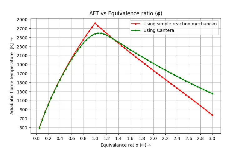
- It can be seen that the peak temperature reported by cantera is lower than that obtained by N-R method with a simple reaction mechanism. This is because cantera solves for each & every intermediate species involved in combustion.
- For very lean combustion where `phi<0.6`, both methods show similar values. This is due to the complete combustion of methane.
- Although AFT predicted by using N-R method is inaccurate, it shows the correct trend for AFT variation with `phi`.
- With a rich mixture, the combustion is incomplete and maximum energy is not released which reduced AFT. In rich combustion contributions from intermediatory reactions increases the AFT which is shown by cantera curve.
PART II
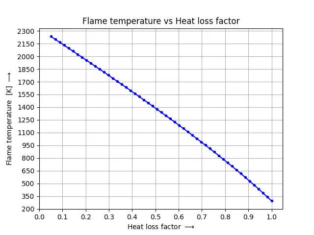
- The plot shows linearly decreasing flame temperature which is expected as heat loss reduces max enthalpy change available during combustion.
PART III
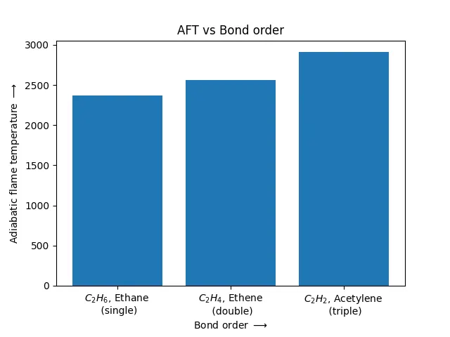
- It is seen that AFT & hence energy released by the type of covalent bond is of order single<double<triple.
- This is because the energy stored by bonds is in order single<double
PART IV
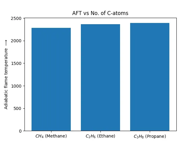
- As the no. of carbon atoms increases so do the no. of covalent bonds. Breaking more bonds per mol of fuel means more energy release per mol.
- More energy release directly implies greater AFT.
- However, the variation in AFT is relatively less compared to AFT variation due to higher-order bonds.