Literature review: ODE Stability

Stability of an ODE:

• Stability, in the context of mathematics, means that a small disturbance in initial conditions doesn't cause any major changes to the system.
• In terms of the solution of a differential equation, a function f(x) is said to be 'stable' if any other solution let's say a numerical solution, of the equation, starts out sufficiently close to it when x = 0 remains close to it for succeeding values of x.
• If the difference between the solutions approaches zero as x increases, the solution is called 'asymptotically stable'.
• If a solution does not have either of these properties, it is called 'unstable'.

Effect on stability engineering simulations:

• The purpose of engineering simulations is to predict the behavior of certain physical phenomena like loads on a body, flow around a body, heat flow, etc.
• These physical phenomena can change rapidly during a simulation and if slight deviations in input to the mathematical model do not have a correspondingly slight effect on the solution, the mathematical equations describing the problem will not accurately model the phenomena.
• If mathematical models blow up the simulation results will be garbage.

Numerical methods to solve a system of ODEs:

Numerical methods for solving ODEs can be classified as linear-multistep and Runge-Kutta methods, implicit and explicit.

Lets us consider a simple ODE,

`" "y'(t) = f(t, y(t))`

Euler's method:

Let's us take the first order forward difference approx. for `y'(t)`,

`" "y'(t) = (y(t + dt) - y(t))/dt`

On re-arranging,

`" "y(t + dt) = y(t) + dt*y'(t)`

`" "therefore y(t +dt) = y(t) + dt*f(t, y(t))`

Here `dt` is the small time interval between times, `t_0, t_1=t_0 + dt, t_2= t_0 + 2*dt,. . .,t_n = t_0 + n*dt`. For the `n^(th)` time step let us denote the approximate value at `(n+1)^(th)` time level as,

`" "y_(n+1) = y_n + dt*f(t_n, y_n)`

In the above equation the RHS is explicitly a function of values of `y` at a previous time level `n`. Hence methods of these kinds are called explicit methods.

Euler's backward method:

This time let us take backward difference approximation for `y(t)`,

`" "y'(t) = (y(t) - y(t-dt))/dt`

On re-arranging,

`" "y(t) = y(t - dt) + dt*y'(t)`

`" "therefore y_n = y_(n - 1) + dt*f( t_n, y_n)`

This equation's RHS is not explicitly a function of `y_(n - 1)`. Hence this is called an implicit equation.

Studying stability of a simple ODE:

Let us take the following ODE and find a solution numerically using python,

`" "dy/dt = - 1000*y - e^(-t)`

By Euler's method,

`" "y_(n +1) = y_n + dt*( - 1000*y_n - e^(-t_n) )" ". . . . (1)`

By Euler' backward method,

`" "y_n = y_(n-1) + dt*( - 1000*t_n - e^(-t_n) )`

`" "therefore y_n = [y_(n -1) - h*e^(-t_n)) / ((1 + 1000*h))" ". . . . (2)`

The analytical solution using integrating factor approach is,

`" "y(t) = c*e^((-1000*t)) - (e^(-t)/999)`

For initial value `y(0) = 0 `,

`" "c = 1 //999`

`" "therefore y(t) = c*e^((-1000*t)) - (e^(-t)/999)" ". . . . (3)`

The code below compares stability by varying `dt` for different schemes,

import numpy as np
import matplotlib.pyplot as plt

# Euler's method (an explicit method)
def f_explicit(dt, t, y):
    return y + dt*(-1000*y - np.exp(-t))

# Euler's backward method (an implicit method)
def f_implicit(dt, t, y):
    return (y - dt*np.exp(-t))/(1 + 1000*dt)

def num_integ(y0, t0, t_end, dt, f):
    y_old       = y0
    t           = t0

    y_new        = []
    i = 0
    while(t <= t_end):
        y_new.append(f(dt, t, y_old))
        y_old = y_new[i]
        t     = t + dt
        i    += 1

    return y_new

# Inputs
y0       = 0
t0       = 0
t_end    = 0.1
dt       = 1.3e-3
y_exp = num_integ (y0, t0, t_end, dt, f = f_explicit)
y_imp = num_integ (y0, t0, t_end, dt, f = f_implicit)

t        = np.arange(t0, t_end, dt)
y_analytical = ( np.exp(-1000*t) - np.exp(-t) )/999

fig, ax = plt.subplots(1,2, figsize = (14,5))

ax[0].plot(t, y_analytical, '-g', label = 'Analytical solution')
ax[0].plot(t, y_exp, '-r', label = 'Approx. by explicit method')
ax[0].set_title(f'For step size {dt:0.3e}')
ax[0].set_xlabel(f't $\longrightarrow$')
ax[0].set_ylabel(f'y ( t ) $\longrightarrow$')
ax[0].legend()

ax[1].plot(t, y_analytical, '-g', label = 'Analytical solution')
ax[1].plot(t, y_imp, '-b', label = 'Approx. by implicit method')
ax[1].set_title(f'For step size {dt:0.3e}')
ax[1].set_xlabel(f't $\longrightarrow$')
ax[1].set_ylabel(f'y ( t ) $\longrightarrow$')
ax[1].legend()

plt.show()

Results & Inferences:

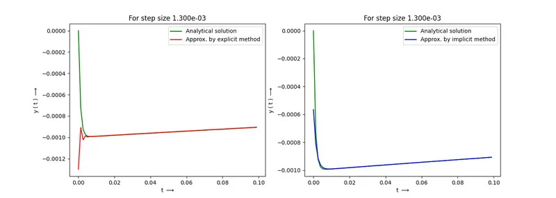
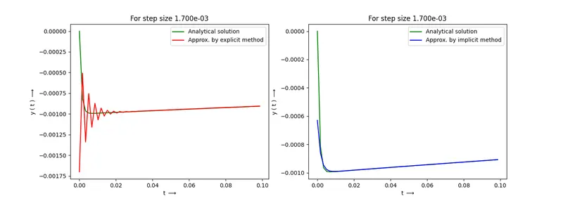
• As seen above, implicit scheme remains stable even for larger time steps.
• The explicit scheme starts showing instability after a certain size of time step.