Flow simulation in a Mixing Tee
# Objective:
The objective of this project is to study the mixing efficiency in a mixing Tee for different lengths of the (main) pipe section and different T-inlet flow velocities.
# Introduction:
The mixing tee is a junction that intersects the main pipe axis at `90^@` from where secondary fluid is added. This component is readily used in processing industries for mixing fluids and its effectiveness is critical for process quality. We will conduct simulations for short & long sections of the main pipe using different T-inlet flow velocities. Then we will compute the average temperature at the outlet and the standard deviation from the mean temperature which is inversely related to the mixing efficiency.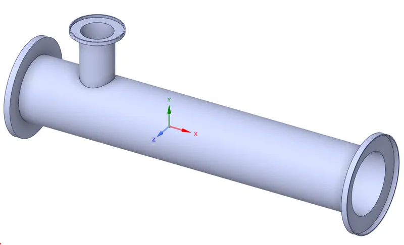
fig.`(1)` : Component geometry
Mixing Tee finds extensive applications in HVAC and petrochemical industries.
# Theory:
- In a mixing Tee, the primary flow is in the main pipe as shown while the secondary flow is added from the T-inlet midway. This causes turbulent mixing of two flows through the rest the of pipe length.
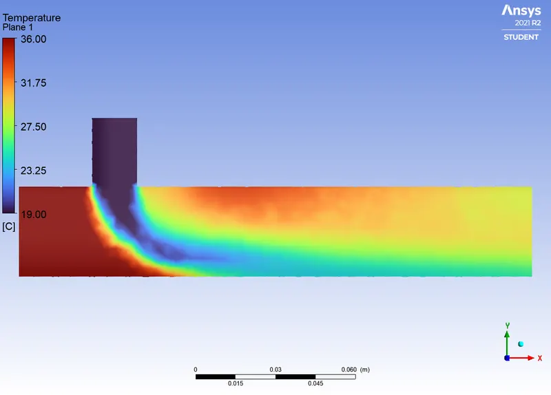
- In this project, we are using hot water (at `36^@C`) in primary flow and cold water (at `19^@C`) through T-inlet so, mixing effectiveness can be quantitatively measured as the standard deviation of temperature at the outlet.
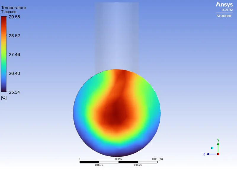
- Thus, a lower standard deviation indicates all particles are closer to the mean temperature and mixing is effective.
# Meshing:
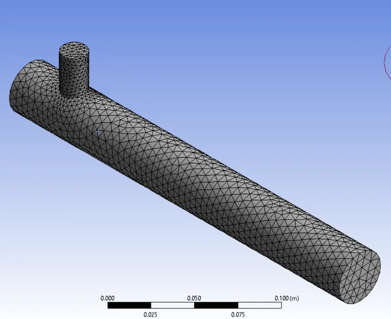
First, we will extract the fluid volume (volume in which flow occurs) from the imported solid model using ANSYS Spaceclaim and then the tetrahedral mesh is generated.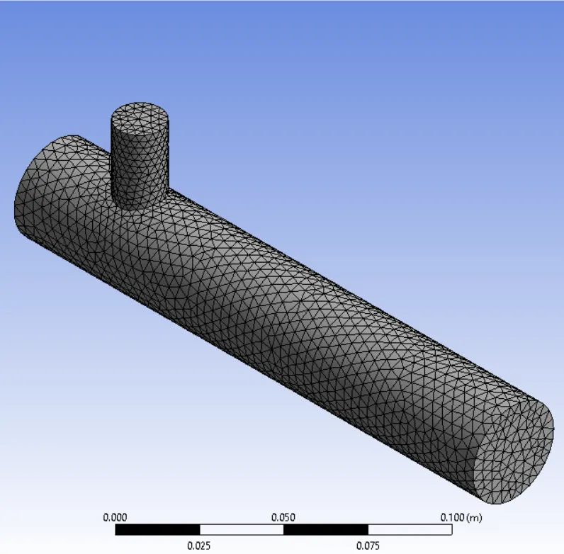
(a)
(b)
fig.`(2)` : Mesh (a)Short & (b)Long pipe.
For meshing, tetrahedral cells are used. The mesh metrics are shown below. Since most cells have quality above 0.7 the meshes are deemed acceptable.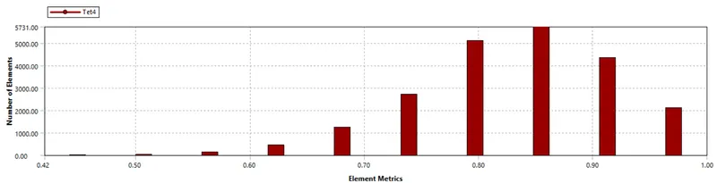
(a)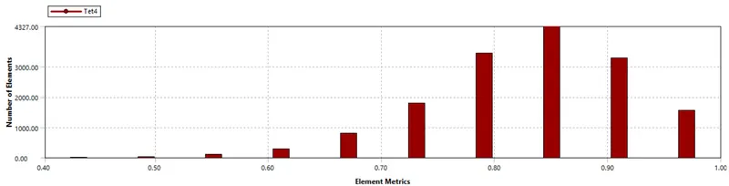
(b)
fig.`(3)` : Mesh metrics (a)Short & (b)Long pipe.
# Solving & modeling the flow:
- The steady-state simulation for turbulent flow will be carried out for short pipe(case-1) and long pipe(case-2) with momentum ratios of 2 & 4 for both cases.
- And the turbulence model (`k-epsilon` & `k-omega` SST) can be decided upon from the simulation results of the first case with momentum ratio 2.
- Also, we are gonna solve the energy equation since we are interested in temperature.
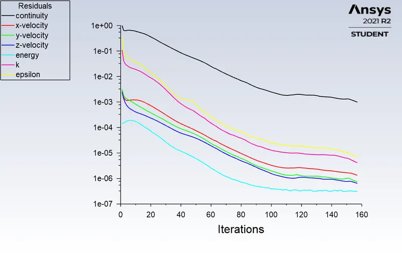
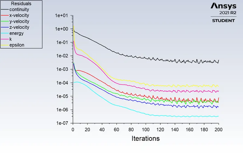
- For hybrid initialization no. of iterations shall be set greater than 14 so that convergence criteria of `1"x"10^(-6)` is reached. We will set no. of iterations to 200.
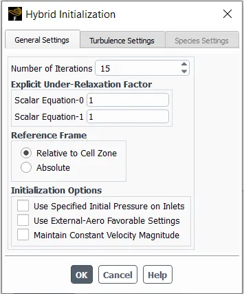
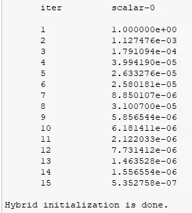
fig.`(4)` : Initialization
# Preliminery simulation results:
(a)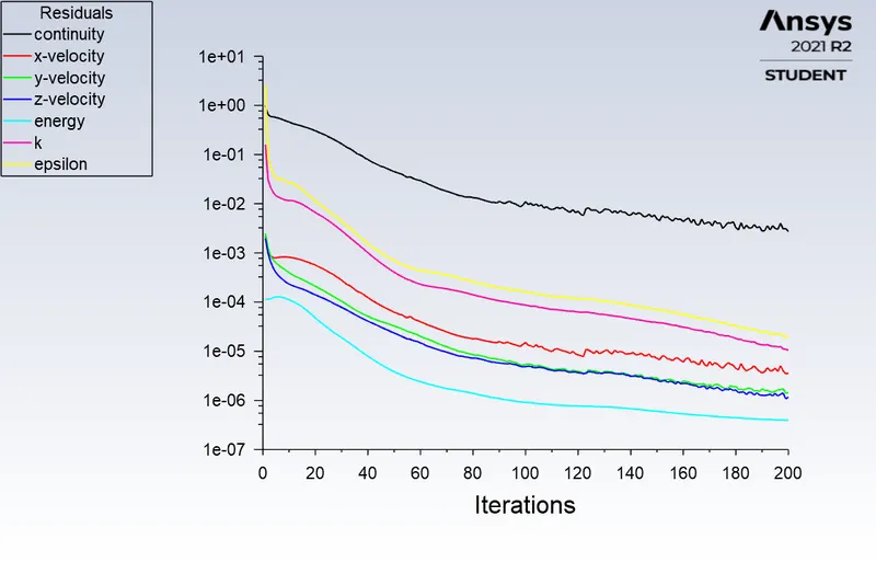
(b)
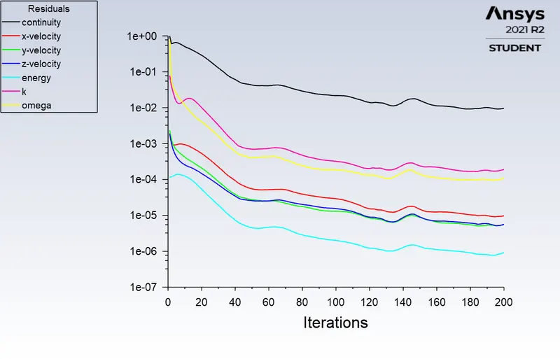
fig.`(5)` : (a) k-`omega` SST & (b) k-`epsilon` turbulence models
- It can be seen that residuals are a bit smaller in the case of `k-epsilon` model & also the amplitude of fluctuation is less with iterations in `k-epsilon` model.
- Also `k-omega` SST model is suitable for capturing near-wall turbulence as well as away from it but since the walls do not interact with the flow in our simulations, k-`epsilon` model is better suited here.
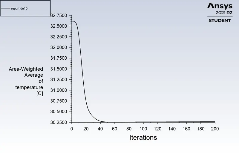
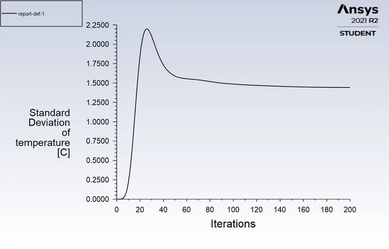
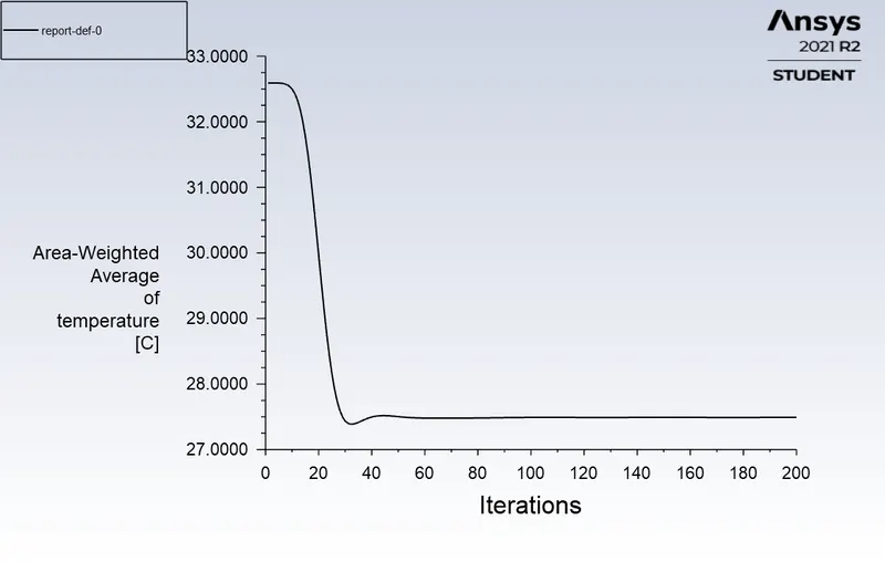
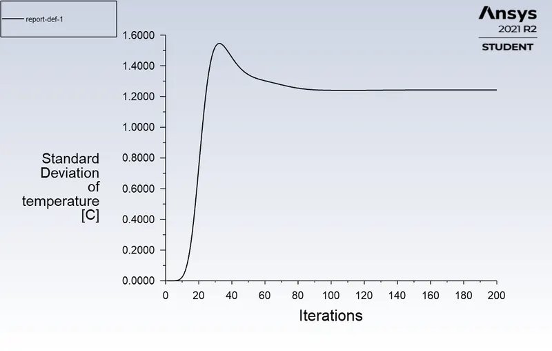
- Also, the above plots of area-weighted average and standard deviation of temperature at outlet indicate that solution has converged to a value. These plots are very much identical for both turbulence models.
# Solving:
- The momentum ratio is defined as,
`"Momentum ratio" = "velocity at cold inlet" / "velocity at hot inlet"`
- We will keep a fixed velocity of `3m//s` at the hot inlet and change cold inlet velocity for varying momentum ratios to 2 & 4.
- Also, the plot of the area-weighted average of temperature and standard deviation of temperature at the outlet will be defined in the reports section for analysis.
- The number of iterations will be set as 200.
# Results & post-processing:
1. Short pipe (Momentum ratio 2)
- Convergence plots
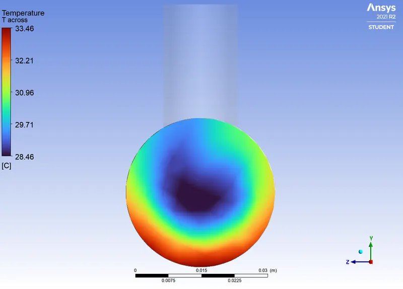
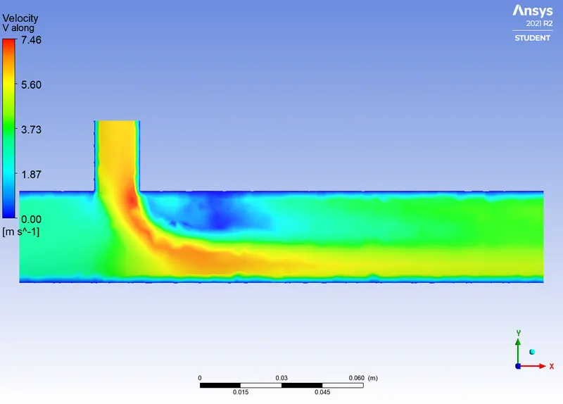
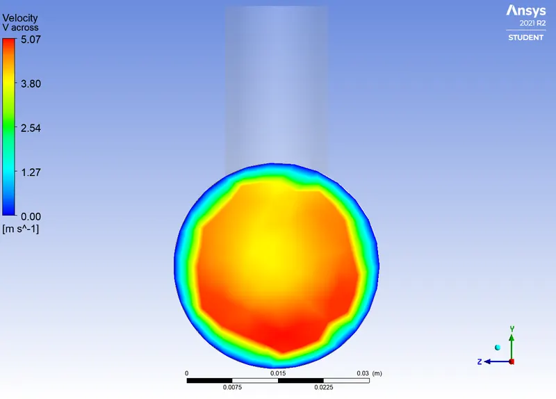
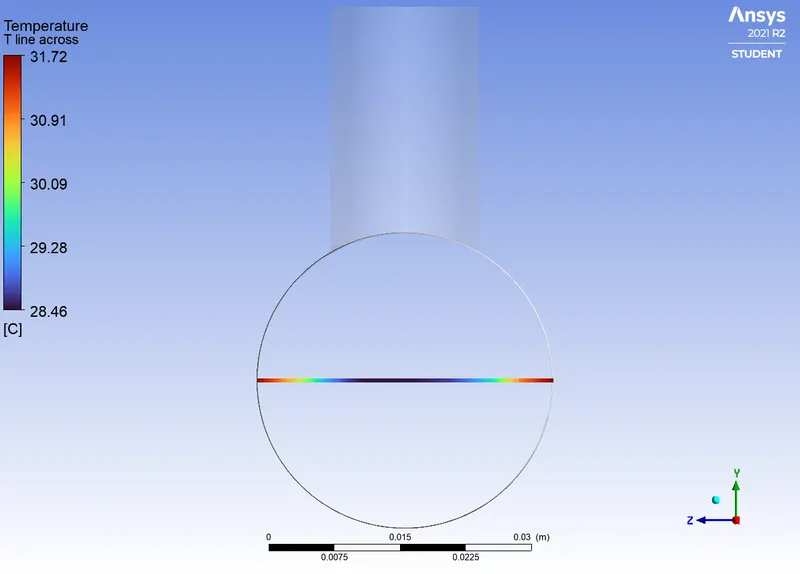
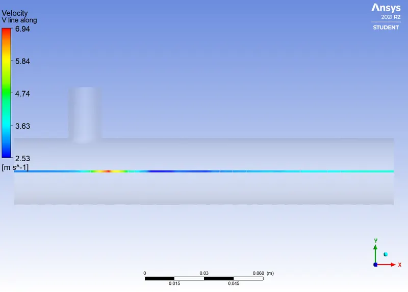
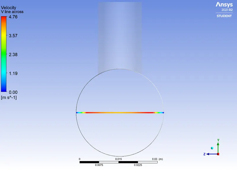
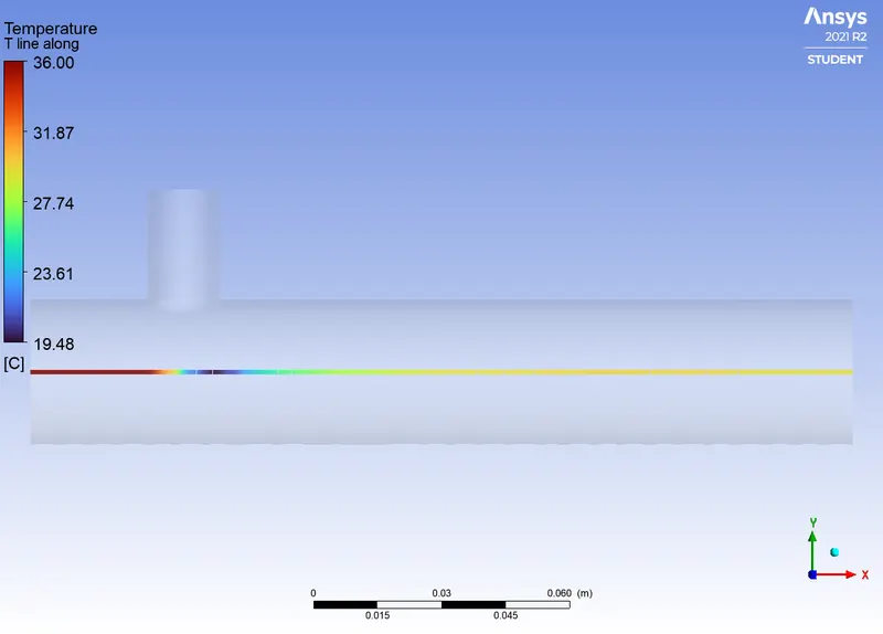
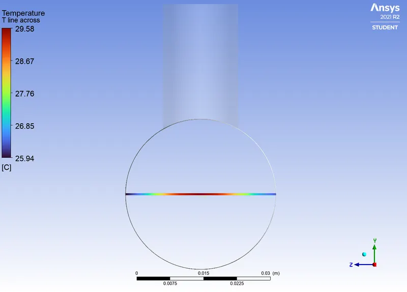
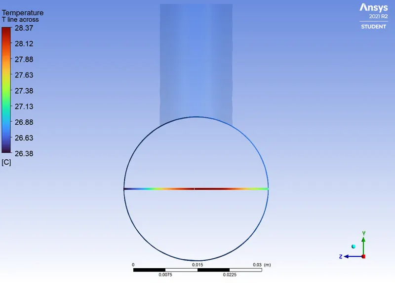
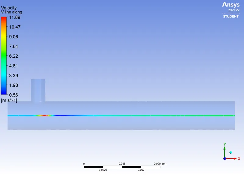
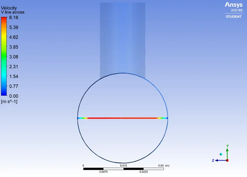
- Temperature and velocity contours plots
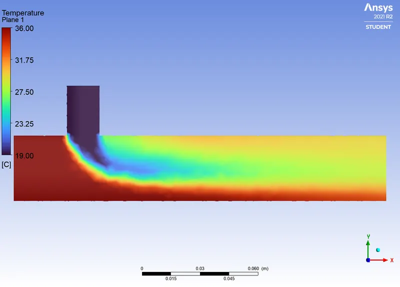
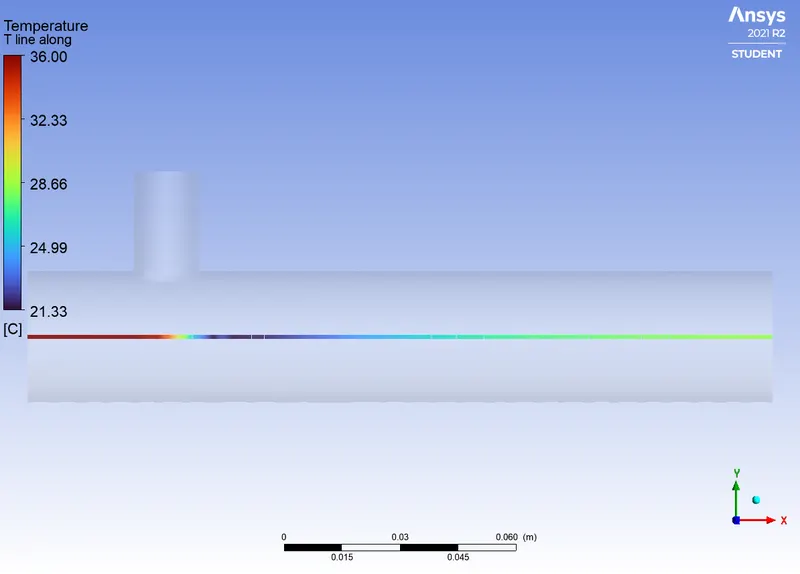
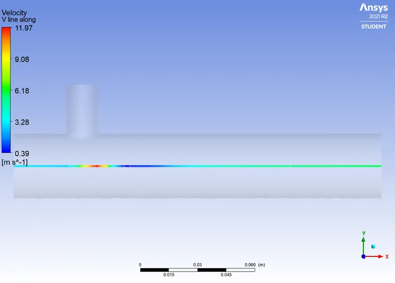
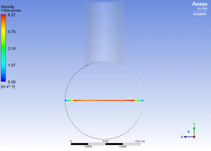
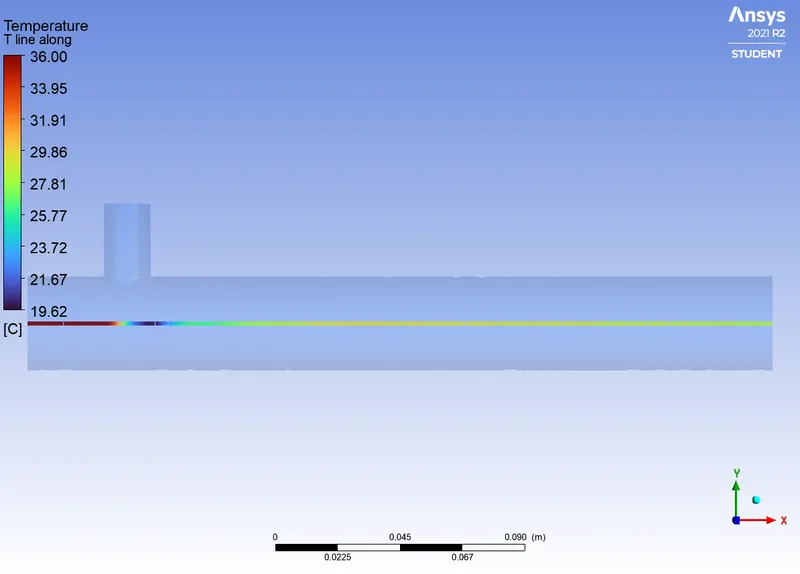
- Temperature and velocity line plots
2. Short pipe (Momentum ratio 4)
- Convergence plots
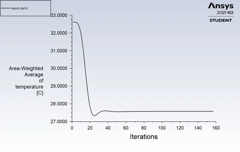
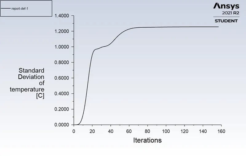
- Temperature and velocity contours plots
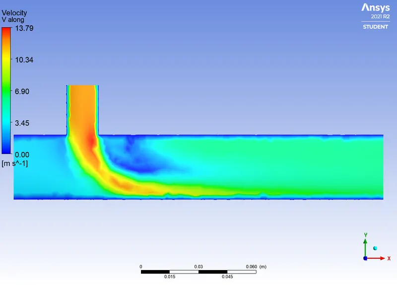
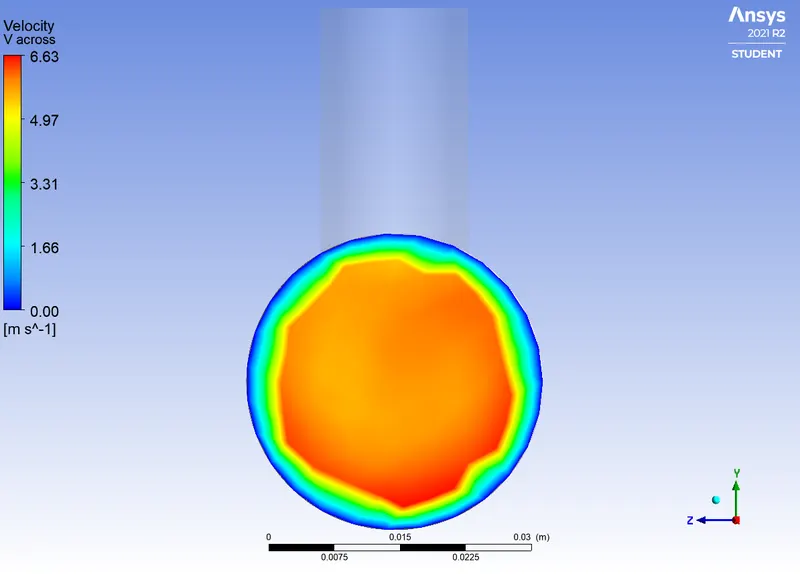
- Temperature and velocity line plots
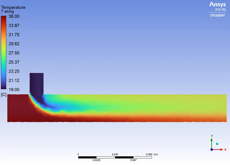
3. Long pipe (Momentum ratio 2)
- Convergence plots
- Temperature and velocity contours plots
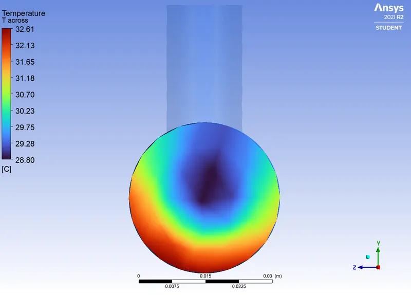
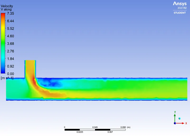
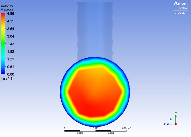
- Temperature and velocity line plots
4. Long pipe (Momentum ratio 4)
- Convergence plots
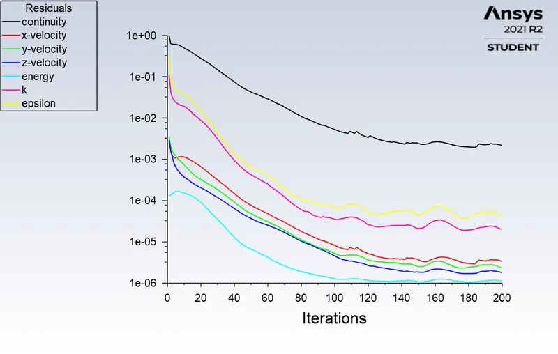
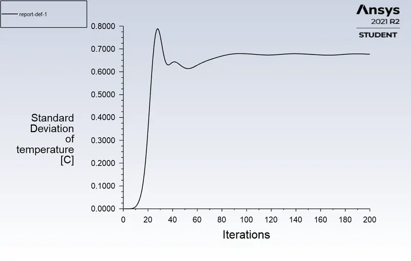
- Temperature and velocity contours plots
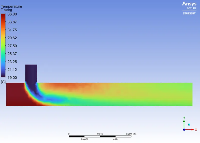
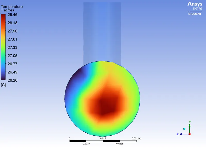
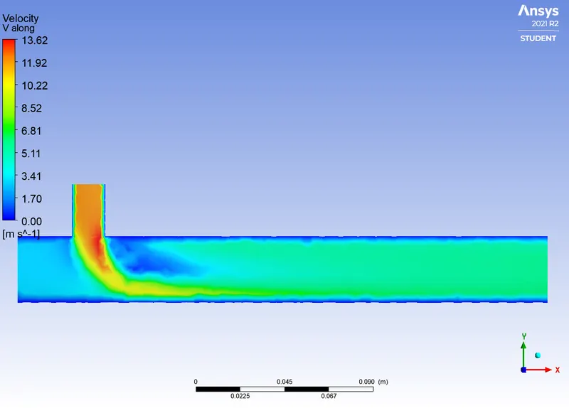
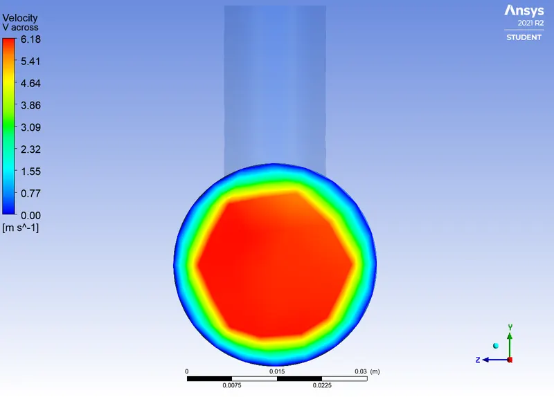
- Temperature and velocity line plots
# Inference:
- The results can be summarised as follows,
| Case |
Momentum Ratio |
Cell Count | Average Temperature at Outlet (in `""^@C` ) | Standard Deviation at Outlet (in `""^@C` ) | Iterations to Converge |
|---|---|---|---|---|---|
| Short pipe | 2 | 21848 | 30.267 | 1.44 | 180-150 |
| 4 | 21848 | 27.577 | 1.256 | 157 | |
| Long pipe | 2 | 15510 | 30.275 | 1.242 | 180-200 |
| 4 | 15510 | 27.492 | 0.677 | 180-200 |
- It can be seen from plots and standard deviation at the outlet that a long pipe indeed mixes flows better than a short pipe.
- The momentum ratio significantly affects mixing effectiveness as standard deviation drops and outlet temperature drops.
# Mesh independence:
- The above study is valid if and only if the solution doesn't change with mesh refinement. We cany out mesh refinement and if the solution doesn't change within a certain margin we say that the solution is independent of mesh.
- For this let us consider the case with the long pipe having a momentum ratio of 2. Mesh refinement was done & the solution was recorded for each refinement in the table below.
| Cell Count | Average Temperature at Outlet (in `""^@C` ) | Percentage change |
|---|---|---|
| 15,510 | 30.275 | - |
| 56,445 | 30.337 | 0.20% |
| 138,811 | 30.352 | 0.05% |
| 506241 | 30.467 | 0.38% |
- Percentage change `<1` is well within tolerance limits for most practical purposes and hence our solution is independent of mesh at this point.
# Conclusion:
- It is established that a longer pipe mix flows better as there is more time and distance for mixing.
- The increased momentum ratio generates greater turbulence leading to better and faster mixing.