FVM Literature Review

Finite Volume Method (FVM) :

In FVM the computational domain is divided into a number of smaller nonoverlapping finite volumes (or cells) and the (integral) governing equations of the flow are solved at (centre & faces) these cells.

Volume integrals in a partial differential equation that contain a divergence term are converted to surface integrals, using the Gauss divergence theorem. These terms are then evaluated as fluxes at the surfaces of each finite volume.

Difference between Finite Volume & Finite Difference Methods :

• FDM uses governing equations in differential form while FVM uses governing equations in integral form.
• In FDM variables are solved at each node while in FVM they are solved at each cell (centre and faces).
• FVM inherently enforces conservation of properties hence it is more reliable than FDM for find solutions with shocks.
• FDM requires function(s) for mapping an unstructured grid to a structured grid which is difficult & tedious to accomplish. In contrast, FVM can be applied directly to unstructured grids without mapping.
• Mesh refinement is easier to implement in FVM, unlike FDM.

For deeper comprehension, let us take the example of 1D steady-state heat conduction through a rod.

The Governing equation needs to be in integral form so,

`" "del/(del x)(alpha (del T)/(del x)) + S = 0" (Differential form)"`

`therefore" "int del/(del x)(alpha (del T)/(del x))dV + int SdV = 0" (Integral form)"`

where,

`alpha = "Thermal diffusivity"`

`S = "Source term"`

In FVM we can divide the rod into nonoverlapping cells with centres `Delta x` distance apart as shown.

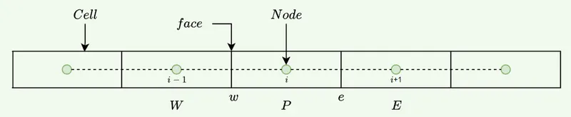
so the equ. becomes,

`" "int_w^e del/(del x)(alpha (del T)/(del x))dAdx + int_w^e SdV = 0" (dA = 1 for 1D)"`

For source term, we will use its average value from `e" to "w`,

`therefore" "[alpha A(del T)/(del x)]_w^e + barSdV = 0`

`therefore" "alpha_w A((del T)/(del x))_w - alpha_e A((del T)/(del x))_e + barSdV = 0`

If source term is a funtion of temprature we can linearize it using Picard's method as,

`" "barS = S^ast + ((del barS)/(del T))^ast (T_P - T_P^ast)" (asterisk denotes current iteration)"`

`" Let, " barS_C = S^ast - ((del barS)/(del T))^ast T_P^ast`

`" & " barS_P = ((del barS)/(del T))^ast`

`therefore" " barS = barS_C + barS_P T_P`

So the discretized governing eqution is,

`therefore" "underbrace(alpha_w A((T_E - T_P)/(Delta x)))_("Heat flux entering") - underbrace(alpha_e A((T_W - T_P)/(Delta x)))_("Heat flux leaving") + underbrace((barS_C + barS_P T_P)dV)_("Source Term") = 0`

Need for interpolation scheme :

• In the finite volume method, quite often we need values of variables on faces (or centres in the case of nodes situated at face centres) where governing equations are not solved.
• So we need to interpolate these values using neighbouring points where the solution is obtained to the required order of accuracy.
• In the above equation, `alpha_w" & "alpha_e` are computed at faces i.e. midway between nodes so, we need to interpolate them.
• Many interpolation schemes are used in FVM. Here we can use quadratic upwind interpolation as, IMAGE `alpha_e = (3alpha_D+6alpha_U-alpha_(UU))//8` and similarly for `alpha_w` we can use the points preceding it(upwind points).

Flux limiter :

• In equ.(1) above, the temperature fluxes can oscillate vigorously near shocks causing the output to get smeared near the shocks.
• To prevent this from happening we put limits on flux oscillations. This way the results are much cleaner near shocks and results provide better reliability.