To determine the thermal efficiency and plot the P-V diagram of Otto cycle.

AIM : To determine the thermal efficiency and plot the P-V diagram of Otto cycle.

PROGRAM : Created using MATLAB.

GOVERNING EQUATIONS :

Boyle's Law

Statement : The volume of a given mass of a gas is inversely related to pressure when the temperature is constant.

V `prop` 1`/` P

PV = Constant

Gay-Lussac's Law

Statement : For a given mass and constant volume of an ideal gas, the pressure exerted on the sides of its container is directly proportional to its absolute temperature.

P `prop` T

P`/`T = Constant

Combined Ideal Gas Laws

P1 V1 `/` T1 = P2 V2 `/` T2

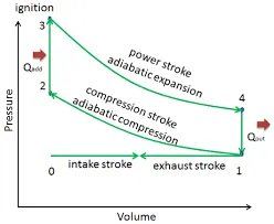
Otto Cycle

Process 0-1 : Intake stroke or Exhaust stroke.

Process 1-2 : Isentropic compression or Compression stroke.

Process 2-3 : Constant volume heat addition.

Process 3-4 : Isentropic expansion or Power stroke.

Process 4-5 : Constant volume heat rejection.

MAIN PROGRAM :

% Program to solve an Otto Cycle and make plots for it.

clear all 
close all 
clc

% Inputs 
gamma = 1.4 ;

% Engine Geometric Parameters 
bore = 0.1 ;
stroke = 0.1 ;
con_rod = 0.15 ;
cr = 12 ;

% Calculating swept and clearance volumes 
v_swept = (pi/4)*bore^2*stroke ;
v_clear = v_swept/(cr-1) ;

% State 1 Variables
P1 = 101325 ;
T1 = 500 ;
V1 = v_swept+v_clear ;

% State 2 Variables
V2 = v_clear ;

% P1V1^gamma = P2V2^gamma 
% P2 = P1*(V1/V2)^gama = P1*(cr)^gamma
P2 = P1*(cr)^gamma ;

% P1V1/T1 = P2V2/T2
T2 = (P2*V2*T1)/(P1*V1) ;

Constant_C = P2*V2^gamma ;
V_Compression = Piston_Kinematics(bore,stroke,con_rod,cr,180,0) ;
P_Compression = Constant_C./(V_Compression).^gamma ;

% State 3 Variables
V3 = V2 ;
T3 = 2300 ;

% P2V2/T2 = P3V3/T3 
% P3 = P2V2T3/T2V3
P3 = (P2*T3)/T2 ;

% State 4 Varibles
V4=V1 ;

% P3V3^gamma = P4V4^gamma
P4 = P3*(V3/V4)^gamma ;

Constant_C = P3*V3^gamma ;
V_Expansion = Piston_Kinematics(bore,stroke,con_rod,cr,0,180) ;
P_Expansion = Constant_C./(V_Expansion).^gamma ;

% Calculation of Thermal Efficiency of Otto Cycle
thermal_efficiency = 1 - (1/(cr)^(gamma-1))


figure(1)
hold on
plot(V1,P1,'*','color','b')
plot(V_Compression,P_Compression)
plot(V2,P2,'*','color','b')
line([V2,V3],[P2,P3])
plot(V3,P3,'*','color','b')
plot(V_Expansion,P_Expansion)
plot(V4,P4,'*','color','b')
line([V4,V1],[P4,P1])
xlabel('Volume')
ylabel('Pressure')

CALLING FUNCTION PROGRAM :

% Deriving calling function called Piston_Kinematics for Otto Cycle program

function [V] = Piston_Kinematics(bore,stroke,con_rod,cr,start_crank,end_crank)

crankpin_rad = stroke/2 ;
R = con_rod/crankpin_rad ;

v_s = (pi/4)*bore^2*stroke ;
v_c = v_s/(cr-1) ;

theta = linspace(start_crank,end_crank,720) ;

term1 = 0.5*(cr-1) ;
term2 = R+1-cosd(theta) ;
term3 = (R^2-sind(theta).^2).^0.5 ;

V = (1+term1*(term2-term3)).*v_c ;

end

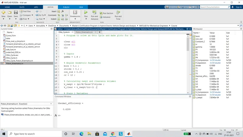
OUTPUT :

PLOTS :

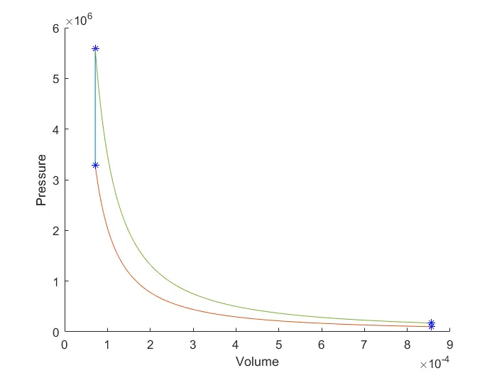
RESULT : The thermal efficiency is found to be 62.99% and the P-V diagram is plotted as shown above.