Project 2 - Rankine cycle Simulator
AIM : To create a Rankine Cycle Simulator using MATLAB.
OBJECTIVES :
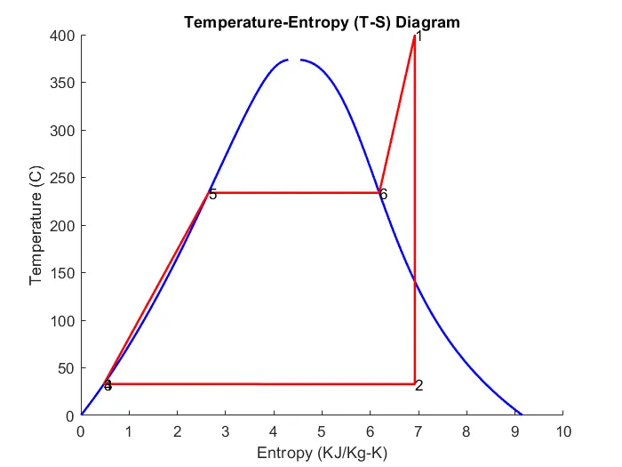
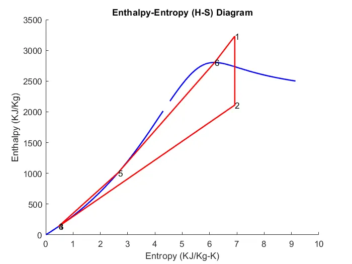
- To plot the T-S and H-S diagrams for the given set of inputs.
- To calculate the various performance characteristics such as Turbine Work, Pump Work, Net Work, Thermal Efficiency, and Specific Steam Consumption.
THEORY :
Rankine cycle is a model used to predict the performance of steam turbine systems. It is also used to study the performance of reciprocating steam engines. It is an idealized thermodynamic cycle of a heat engine that converts heat into mechanical work while undergoing phase change. It is an idealized cycle in which friction losses in each of the four components are neglected.
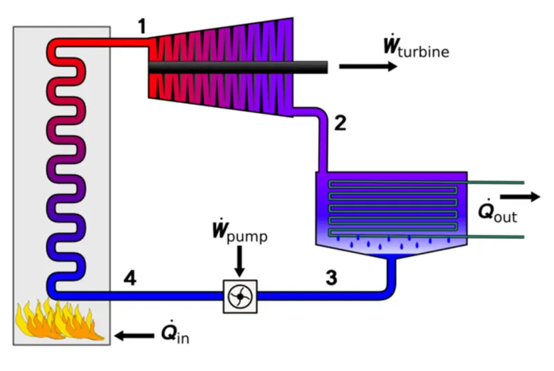
The four processes in the Rankine Cycle are as follows :
Process 1-2 : Isentropic Expansion in the Turbine.
In this process the dry saturated vapour expands through a turbine, generating power. This decreases the temperature and pressure of the vapour, and some condensation may occur.
Process 2-3 : Constant Pressure Heat Rejection by the Condenser.
From the turbine,the wet vapour then enters a condenser, where it is condensed at a constant pressure to become a saturated liquid.
Process 3-4 : Isentropic Compression in the Pump.
The working fluid is pumped from low to high pressure. As the fluid is a liquid at this stage, the pump requires little input energy.
Process 4-1 : The high-pressure liquid enters a boiler, where it is heated at constant pressure by an external heat source to become a dry saturated vapour.
BLOCK DIAGRAM :
GOVERNING EQUATIONS :
Turbine Work (KJ/Kg) : Wt = h1 - h2
where h1 : Enthalpy at State 1
h2 : Enthalpy at State 2
Pump Work (KJ/Kg) : Wp = h4 - h3
where h3 : Enthalpy at State 3
h4 : Enthalpy at State 4
Net Work (KJ/Kg) : Wnet = Wt - Wp
Thermal Efficiency : Nthermal = Wnet/Qin
where Qin is the heat input from the boiler = h1 - h4
Specific Steam Consumption (Kg/KW-h) : SSC = 3600/Wnet
PROGRAM : The code is written using MATLAB.
% Rankine Cycle Simulator

clear all
close all
clc

% Displaying various processes
disp('Rankine Cycle Simulator')
disp('Process 1-2 : Isentropic expansion in the turbine')
disp('Process 2-3 : Constant pressure heat rejection by the condenser')
disp('Process 3-4 : Isentropic Compression in the pump')
disp('Process 4-1 : Constant pressure heat addition by the boiler')

% Inputs

% Turbine Inlet Temperature (C)
t1 = input('Enter the temperature at the turbine inlet (in Degree Celsius) = ');
% Turbine Inlet Pressure (Bar)
p1 = input('Enter the pressure at the turbine inlet (in Bar) = ');
% Turbine Outlet Pressure (Bar) = Condenser Inlet Pressure (Bar)
p2 = input('Enter the pressure at the condenser intlet (in Bar) = ');

% Process 1-2 : Isentropic expansion in the turbine

% Enthalpy (KJ/Kg)
h1 = XSteam('h_pT',p1,t1);
% Entropy (KJ/Kg-K)
s1 = XSteam('s_pT',p1,t1);

% Process 2-3 : Constant pressure heat rejection by the condenser

% Entropy (KJ/Kg-K)
s2 = s1;
% Vapour Fraction (s = sf+x(sg-sf))
sf = XSteam('sL_p',p2);
sg = XSteam('sV_p',p2);
x2 = (s2-sf)/(sg-sf);
% Enthalpy (KJ/Kg) (h = hf+x(hg-hf))
hf = XSteam('hL_p',p2);
hg = XSteam('hV_p',p2);
h2 = hf+(x2*(hg-hf));
% Temperature (C)
t2 = XSteam('Tsat_p',p2);

% Process 3-4 : Isentropic Compression in the pump

% Pressure
p3 = p2;
% Enthalpy (KJ/Kg)
h3 = XSteam('hL_p',p3);
% Entropy (KJ/Kg-K)
s3 = XSteam('sL_p',p3);
% Temperature (C)
t3 = XSteam('T_hs',h3,s3);

% Process 4-1 : Constant pressure heat addition by the boiler

% Pressure
p4 = p1;
% Specific Volume
vf = XSteam('vL_p',p3);
% Pump Work (KJ/Kg)
Wp = (vf*(p4-p3)*10^5)/10^3;
% Enthalpy (KJ/Kg)
h4 = Wp+h3;
% Entropy (KJ/Kg-K)
s4 = XSteam('s_ph',p4,h4);
% Temperature (C)
t4 = XSteam('T_hs',h4,s4);

% State 5 Variables
p5 = p4;
t5 = XSteam('Tsat_p',p5);
h5 = XSteam('hL_p',p5);
s5 = XSteam('sL_p',p5);

% State 6 Variables
t6 = t5;
p6 = XSteam('psat_T',t6);
h6 = XSteam('hV_T',t6);
s6 = XSteam('sV_T',t6);

% Calculating various performance characteristics

% Turbine Work (KJ/Kg)
Wt = h1-h2;

% Net Work (KJ/Kg)
Wnet = Wt-Wp;

% Boiler Heat Output (KJ/Kg)
Q1 = h1-h4;

% Condenser Heat Output (KJ/Kg)
Q2 = h2-h3;

% Thermal Efficiency
Nthermal = (Wnet/Q1)*100;

% Specific Steam Consumption (Kg/KW-h)
SSC = 3600/Wnet;

% Plotting Temperature-Entropy (T-S) Diagram

% Plotting Saturation Curve
tsat1 = linspace(0,374,1000);
for i = 1:length(tsat1)
    ssc1(i) = XSteam('sL_T',tsat1(i));
end
for j = 1:length(tsat1)
    ssc2(j) = XSteam('sV_T',tsat1(j));
end

figure(1)
hold on
plot([ssc1 ssc2],[tsat1 tsat1],'linewidth',1.5,'color','b')
plot([s1 s2 s3 s4 s5 s6 s1],[t1 t2 t3 t4 t5 t6 t1],'linewidth',1.5,'color','r')
text(s1,t1,'1')
text(s2,t2,'2')
text(s3,t3,'3')
text(s4,t4,'4')
text(s5,t5,'5')
text(s6,t6,'6')
title('Temperature-Entropy (T-S) Diagram')
xlabel('Entropy (KJ/Kg-K)')
ylabel('Temperature (C)')

% Plotting Enthalpy-Entropy (H-S) Diagram

% Plotting Saturation Curve
tsat1 = linspace(0,374,1000);
for i = 1:length(tsat1)
    hsc1(i) = XSteam('hL_T',tsat1(i));
end
for j = 1:length(tsat1)
    hsc2(j) = XSteam('hV_T',tsat1(j));
end

figure(2)
hold on
plot([ssc1 ssc2],[hsc1 hsc2],'linewidth',1.5,'color','b')
plot([s1 s2 s3 s4 s5 s6 s1],[h1 h2 h3 h4 h5 h6 h1],'linewidth',1.5,'color','r')
text(s1,h1,'1')
text(s2,h2,'2')
text(s3,h3,'3')
text(s4,h4,'4')
text(s5,h5,'5')
text(s6,h6,'6')
title('Enthalpy-Entropy (H-S) Diagram')
xlabel('Entropy (KJ/Kg-K)')
ylabel('Enthalpy (KJ/Kg)')

% Displaying the Output

% State 1
fprintf('At State Point 1 :\r\n')
fprintf('P1 is : %f Bar\r\n',p1)
fprintf('T1 is : %f C\r\n',t1)
fprintf('H1 is : %f KJ/Kg\r\n',h1)
fprintf('S1 is : %f KJ/Kg-K\r\n',s1)

% State 2
fprintf('At State Point 2 :\r\n')
fprintf('P2 is : %f Bar\r\n',p2)
fprintf('T2 is : %f C\r\n',t2)
fprintf('H2 is : %f KJ/Kg\r\n',h2)
fprintf('S2 is : %f KJ/Kg-K\r\n',s2)
fprintf('X2 is : %f \r\n',x2)

% State 3
fprintf('At State Point 3 :\r\n')
fprintf('P3 is : %f Bar\r\n',p3)
fprintf('T3 is : %f C\r\n',t3)
fprintf('H3 is : %f KJ/Kg\r\n',h3)
fprintf('S3 is : %f KJ/Kg-K\r\n',s3)

% State 4
fprintf('At State Point 4 :\r\n')
fprintf('P4 is : %f Bar\r\n',p4)
fprintf('T4 is : %f C\r\n',t4)
fprintf('H4 is : %f KJ/Kg\r\n',h4)
fprintf('S4 is : %f KJ/Kg-K\r\n',s4)

% Performance Characteristics

% Turbine Work
fprintf('Wt is : %f KJ/Kg\r\n',Wt)

% Pump Work
fprintf('Wp is : %f KJ/Kg\r\n',Wp)

% Net Work
fprintf('Wnet is : %f KJ/Kg\r\n',Wnet)

% Thermal Efficiency
fprintf('Nthermal is : %f Percent\r\n',Nthermal)

% Specific Steam Consumption
fprintf('SSC is : %f Kg/KW-h\r\n',SSC)
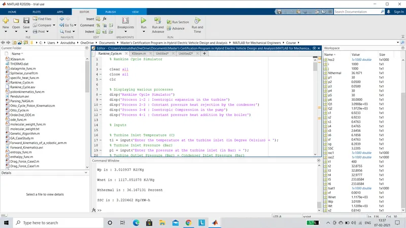
OUTPUT :
Rankine Cycle Simulator
Process 1-2 : Isentropic expansion in the turbine
Process 2-3 : Constant pressure heat rejection by the condenser
Process 3-4 : Isentropic Compression in the pump
Process 4-1 : Constant pressure heat addition by the boiler
Enter the temperature at the turbine inlet (in Degree Celsius) = 400
Enter the pressure at the turbine inlet (in Bar) = 30
Enter the pressure at the condenser intlet (in Bar) = 0.05
At State Point 1 :

P1 is : 30.000000 Bar

T1 is : 400.000000 C

H1 is : 3231.571027 KJ/Kg

S1 is : 6.923259 KJ/Kg-K

At State Point 2 :

P2 is : 0.050000 Bar

T2 is : 32.875490 C

H2 is : 2110.708212 KJ/Kg

S2 is : 6.923259 KJ/Kg-K

X2 is : 0.814256

At State Point 3 :

P3 is : 0.050000 Bar

T3 is : 32.895584 C

H3 is : 137.765119 KJ/Kg

S3 is : 0.476254 KJ/Kg-K

At State Point 4 :

P4 is : 30.000000 Bar

T4 is : 32.977721 C

H4 is : 140.776056 KJ/Kg

S4 is : 0.476470 KJ/Kg-K

Wt is : 1120.862815 KJ/Kg

Wp is : 3.010937 KJ/Kg

Wnet is : 1117.851878 KJ/Kg

Nthermal is : 36.167131 Percent

SSC is : 3.220462 Kg/KW-h
PLOTS :
T-S Diagram :
H-S Diagram :
EXPLANATION :
- We begin by writing the code to display the name of the simulator and the various processes under it using the 'disp' command.
- Now we write the code to receive the inputs from the user for Turbine Inlet Pressure, Turbine Inlet Temperature and Condenser Inlet Presssure.These values are assigned to 3 different variables.
- The values of Enthalpy,Entropy and Temperature for the various processes are obtained by calling the 'XSteam' file.Also thermodynamic equations are used to calculate other required variables.
- In order to plot the saturation curve we have to consider a range of saturation temperatures from 0 to 374 using the 'linspace' command.Now using the 'for loop' the values of Entropy and Enthalpy are determined for varying values of saturation temperatures.The values of Entropy and Enthalpy are determined at both liquid and vapour phase.
- Now the graphs for T-S and H-S Diagrams are plotted using the 'plot' command.The 'text' command is used to represent various State Points in the plots.Also the 'title' command is used to display the title of the graph.The 'xlabel' and 'ylabel' commands are used to represent the X and Y axes.
- Finally in order to display the variables at different state points and the performance charateristics in the command window we use the 'fprintf' command.
REFERENCES :