Final Project: Electric Rickshaw modelling
AIM : To create a MATLAB model of an electric rickshaw.
OBJECTIVES :
- The electric rickshaw should be rear wheel driven, powered by a PM brushed type motor.
- Efficiency points of the motor controller and motor should be assumed.
- An excel sheet of all input and assumed data should be depicted.
- For any three standard driving cycles, the energy consumption and temperature rise of the motor & controller should be determined.
INTRODUCTION :
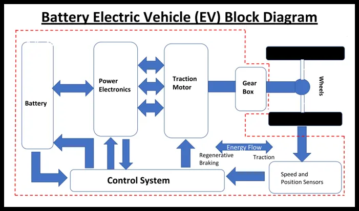
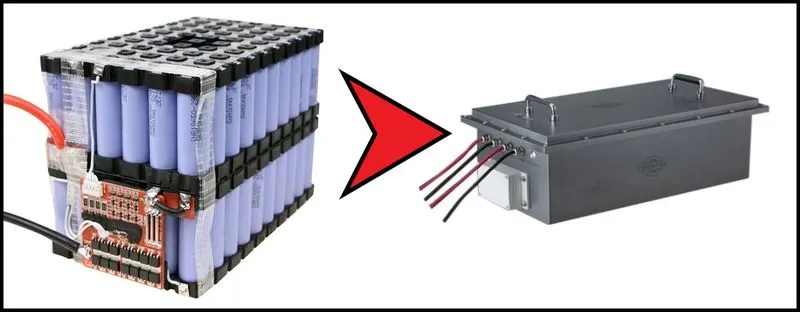
Battery Pack : The function of the battery in an electric car is as an electrical energy storage system in the form of direct-current electricity (DC). If it gets a signal from the controller, the battery will flow DC electrical energy to the inverter to then be used to drive the motor. The type of battery used is a rechargeable battery that is arranged in such a way as to form what is called a traction battery pack.There are various types of electric car batteries. The most widely used is the type of lithium-ion batteries.
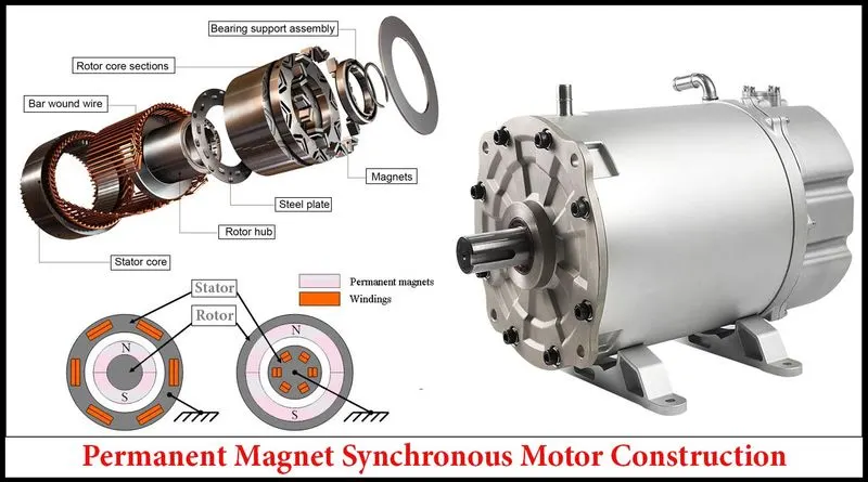
Electric Traction Motor : Since the controller provides electrical power from the traction battery, the electric traction motors will work turning the transmission and wheels. Some hybrid electric cars use a type of generator-motor that performs the functions of propulsion and regeneration. In general, the type of electric motor used is the BLDC (brushless DC) motor.
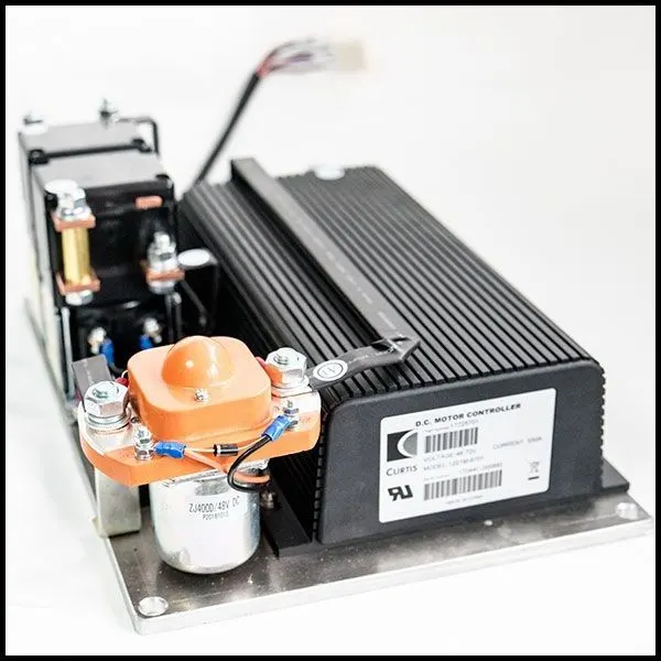
Controller : The main function of the controller is as a regulator of electrical energy from batteries and inverters that will be distributed to electric motors. While the controller itself gets the main input from the car pedal (which is set by the driver). This pedal setting will determine the frequency variation or voltage variation that will enter the motor, and at the same time determine the car’s speed.In brief, this unit manages the flow of electrical energy delivered by the traction battery, controlling the speed of the electric traction motor and the torque it produces. This component will determine how electric car work.
Power Electronics : In electric cars, power electronics is responsible for converting and controlling electric power in the system. These include inverter, converter, and on-board charger. Operations at high voltage or high current can be efficiently executed by utilizing power electronic devices, as they deliver faster switching rate at higher efficiency. In addition, power electronics control both unidirectional as well as bidirectional flow of energy, depending on the usage, and the regenerated energy can be sent back to utility.Power electronic is a key technology used in various applications to optimize energy management, providing the conversion to operate motors, battery storage, and generators. Complex power electronics are represented as the interconnection of conversion blocks in AC/DC, DC/AC, DC/DC, and AC/AC.Power electronics is used in EV that require high power electric energy to rotate the electric motors. Power modules reduce power loss, owing to their high frequency. In addition, the components such as silicon-based power MOSFETs and IGBTs are used as power electronic switches in the power train automotive electric and electronic systems for reducing the overall size.
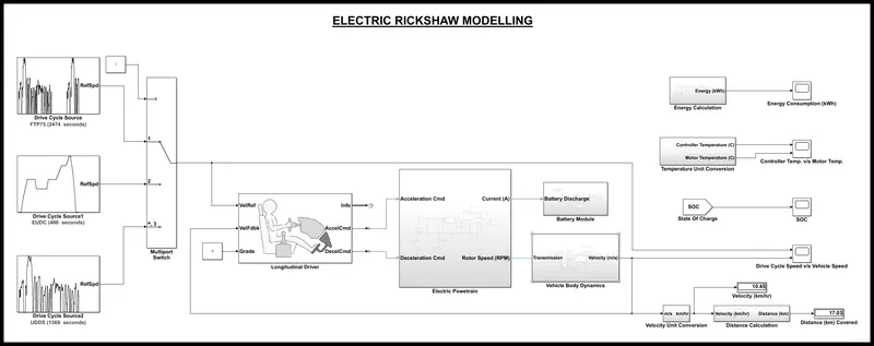
MATLAB SIMULINK MODEL OF PURE ELECTRIC RICKSHAW
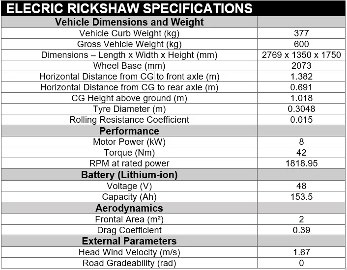
ASSUMED DATA
INDIVIDUAL SUB-SYSTEMS
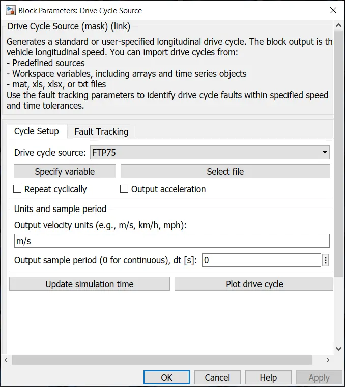
Drive Cycle Source
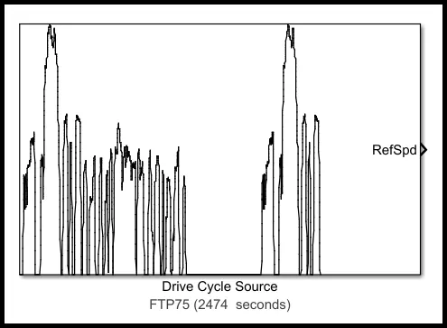
This block generates a standard or user-specified longitudinal drive cycle. The block output is the specified vehicle longitudinal speed, which you can use to:
-
Predict the engine torque and fuel consumption that a vehicle requires to achieve desired speed and acceleration for a given gear shift reference.
-
Produce realistic velocity and shift references for closed loop acceleration and braking commands for vehicle control and plant models.
-
Study, tune, and optimize vehicle control, system performance, and system robustness over multiple drive cycles.
-
Identify the faults within tolerances specified by standardized tests, including:
-
EPA dynamometer driving schedules.
-
Worldwide Harmonised Light Vehicle Test Procedure (WLTP) laboratory tests.
-
For the drive cycles, you can use :
-
Drive cycles from predefined sources. By default, the block includes the FTP-75 drive cycle. Additional drive cycles can be installed from a support package. The support package has drive cycles that include the gear shift schedules, for example JC08 and CUEDC.
-
Workspace variables.
-
.mat, .xls, .xlsx, or .txt files.
-
Wide open throttle (WOT) parameters, including initial and nominal reference speed, deceleration start time, and final reference speed.
With reference to this model :
We have considered FTP-75, EUDC and UDDS Drive Cycles for testing the EV rickshaw performance characteristics.
Longitudinal Driver
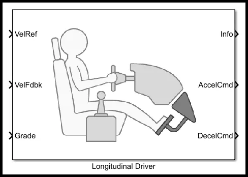
This block implements a longitudinal speed-tracking controller. Based on reference and feedback velocities, the block generates normalized acceleration and braking commands that can vary from 0 through 1. You can use the block to model the dynamic response of a driver or to generate the commands necessary to track a longitudinal drive cycle.
External Actions parameters can be used to create input ports for signals that can disable, hold, or override the closed-loop acceleration or deceleration commands. The block uses this priority order for the input commands: disable (highest), hold, override.
With reference to this model :
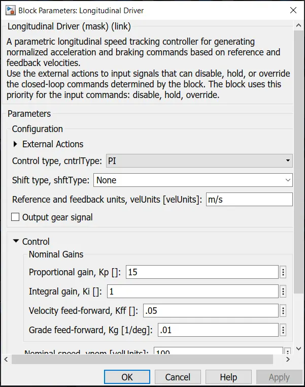
We have not considered any external actions to simplify the model.
The controller type is set to Proportional-integral (PI) control with tracking windup and feed-forward gains.The Proportional Gain (Kp) and the Integral Gain (Ki) are set at default values.This tuning of the controller is done to help the vehicle follow the Drive Cycle to the greatest possible extent.

The shift type is set to none which represents 'No transmission'. Block outputs a constant gear of 1.This setting is used to minimize the number of parameters we need to generate acceleration and braking commands to track forward vehicle motion. This setting does not allow reverse vehicle motion.
Electric Motor Drive
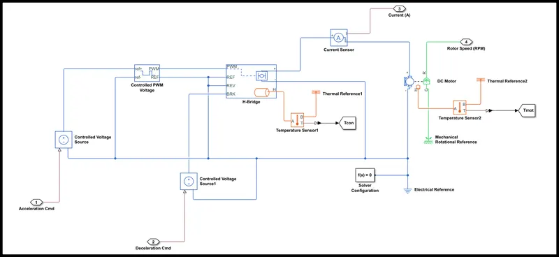
Controlled Voltage Source : This block represents an ideal voltage source that is powerful enough to maintain the specified voltage at its output regardless of the current flowing through the source.The output voltage is V = Vs, where Vs is the numerical value presented at the physical signal port.The block has one physical signal input port and two electrical conserving ports associated with its electrical terminals.
With reference to this model :
We have used two Controlled Voltage Source blocks.The outputs associated with the Longitudinal Driver is fed as input to each of the two Controlled Voltage Source blocks, through the physical signal input port.The Controlled Voltage Source blocks generate an output voltage proportional to the Acceleration and Deceleration signals provided by the Longitudinal Driver.
The positive terminal of the Controlled Voltage Source block provided with Acceleration input signal is connected to the positive reference of the Controlled PWM Voltage block, whereas the negative terminal is grounded to an Electrical Reference block.
The negative terminal of the Controlled Voltage Source block provided with Deceleration input signal is connected to the Brake port of the H-Bridge block, whereas the negative terminal is grounded to an Electrical Reference block.
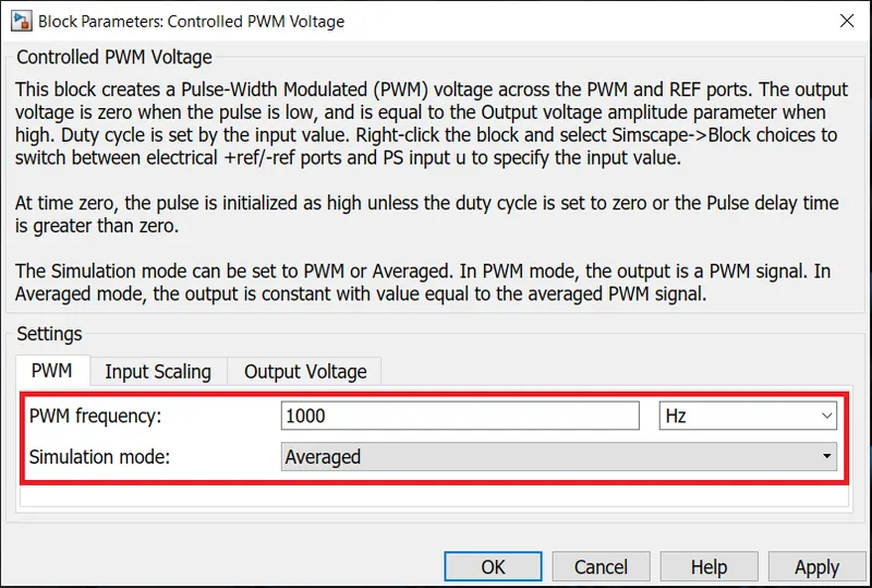
Controlled PWM Voltage : This block represents a pulse-width modulated (PWM) voltage source.It creates a Pulse-Width Modulated (PWM) voltage across the PWM and REF ports.The block calculates the duty cycle based on the reference voltage across its ref+ and ref- ports.The output voltage is zero when the pulse is low, and is equal to the Output voltage amplitude parameter when high.
With reference to this model :
We have set the simulation mode to 'Average' to speed up simulations.This applies the average of the demanded PWM voltage to the motor. The Averaged mode assumes that the impedance of the motor inductive term is small at the PWM frequency.Averaged mode also helps in linearising the model.We can only linearize the block for inputs corresponding to a duty cycle greater than zero and less than 100 percent.
H-Bridge : The H-Bridge block represents a H-bridge motor driver. The block has the following two Simulation mode options:
1. PWM — The H-Bridge block output is a controlled voltage that depends on the input signal at the PWM port. If the input signal has a value greater than the Enable threshold voltage parameter value, the H-Bridge block output is on and has a value equal to the value of the Output voltage amplitude parameter. If it has a value less than the Enable threshold voltage parameter value, the block maintains the load circuit using one of the following three Freewheeling mode options:
-
Via one semiconductor switch and one freewheeling diode.
-
Via two freewheeling diodes.
-
Via two semiconductor switches and one freewheeling diode.
The first and third options are sometimes referred to as synchronous operation.
The signal at the REV port determines the polarity of the output. If the value of the signal at the REV port is less than the value of the Reverse threshold voltage parameter, the output has positive polarity; otherwise, it has negative polarity.
2. Averaged — This mode has two Load current characteristics options:
-
Smoothed
-
Unsmoothed or Discontinuous.
The block has an optional thermal port, hidden by default. To expose the thermal port, right-click the block in your model, and then from the context menu select Simscape > Block choices > Show thermal port. This action displays the thermal port H on the block icon, and adds the Temperature Dependence and Thermal Port parameters.
When the thermal port is visible:
-
The heat generated by the bridge on-resistance and freewheeling diodes is added to the thermal port. The thermal port has an associated thermal mass and initial temperature that you can set from the Thermal Port parameters.
-
The bridge on-resistance and freewheeling diode resistance become functions of temperature. You can define the values for these resistances and the second measurement temperature from the Temperature Dependence parameters. Resistance is assumed to vary linearly between the two measurement temperatures. Extrapolation is used for temperatures outside of this range, except for when simulating in averaged mode with discontinuous load current characteristics.
With reference to this model :
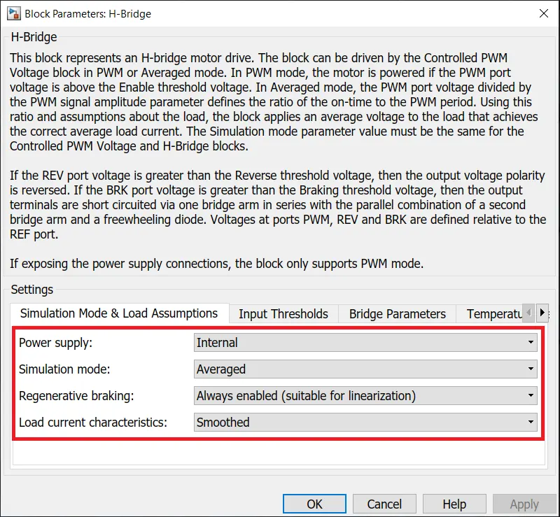
We have set the Simulation mode parameter to 'Averaged' to speed up simulations when driving the H-Bridge block with a Controlled PWM Voltage block. We must also set the Simulation mode parameter of the Controlled PWM Voltage block to Averaged mode. This applies the average of the demanded PWM voltage to the motor. The accuracy of the Averaged mode simulation results relies on the validity of our assumption about the load current.
We have set the Power Supply to be 'Internal' and set the Load Current Characteristics to be 'Smoothed'.
We have also enabled 'Regenerative Braking' so that the DC motor can function as a generator during braking and thus help in recharging the battery.
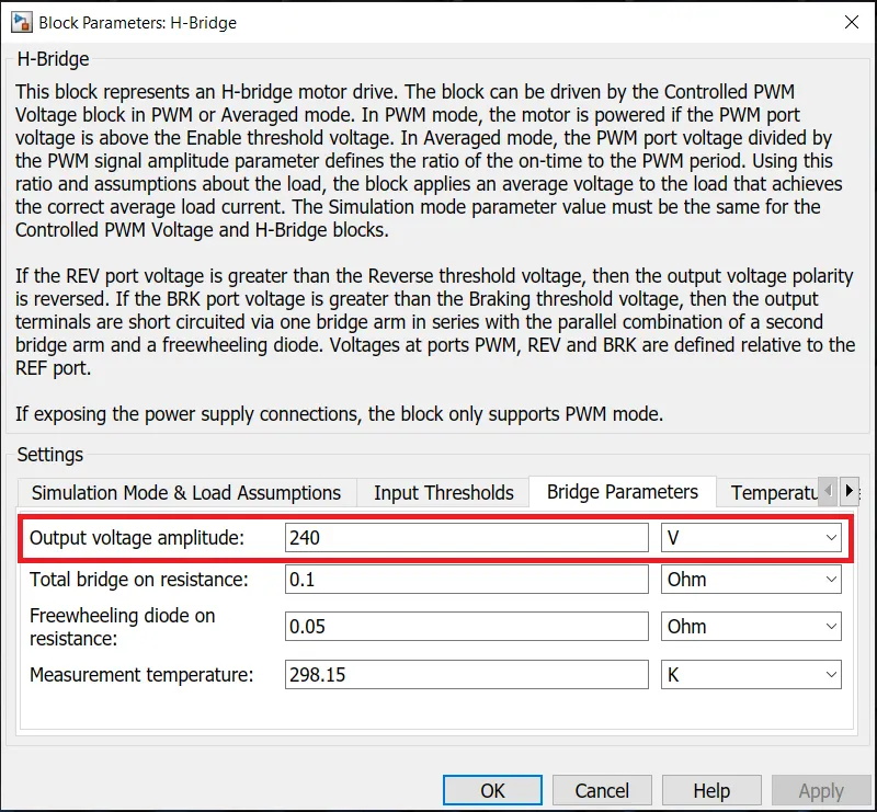
The output voltage amplitude of the H-Bridge is set to 240 V.
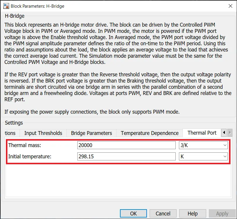
Since we have enabled the thermal port, it is necessary to determine the thermal mass and the initial temperature of the H-bridge motor controller.The thermal mass is set to 20000 J/K from the default value of 100 J/K, whereas the initial temperature is kept default at 298.15 K or 25 C.
Thermal mass represents the energy required to raise the temperature of the thermal port by one degree.Hence by increasing the thermal mass to a value of 20000 J/K, 20000 Joules heat has to be absorbed by the H-bridge for its temperature to rise by 1 K.
The reason for increasing the thermal mass to a very high value of 20000 J/K is to improve the performance of the H-bridge.
Electronic components including solid state devices, resistors, capacitors, inductors and others are all susceptible to failure from overheating. The expected life of any component, and of any final product built from those components, is affected by the temperature at which they operate. In fact, a temperature increase of 10 degrees Centigrade is generally accepted as cutting the life of a device in half. Likewise, reducing the temperature by 10 degrees can double its expected life.
We know that increase in temperature results in the increase in resistance, thereby degrading the performance of the power electronics present in the H-bridge.
Hence by increasing the thermal mass to a very high value, we can reduce the rate of rise in temperature of the H-bridge.
Thus we can make sure that the temperature of the H-bridge does not cross the pre-defined limits, thereby not allowing the efficiency of the H-bridge to drop.
DC Motor : This block represents the electrical and torque characteristics of a DC motor.The block assumes that no electromagnetic energy is lost, and hence the back-emf and torque constants have the same numerical value when in SI units.When a positive current flows from the electrical + to - ports, a positive torque acts from the mechanical C to R ports. Motor torque direction can be changed by altering the sign of the back-emf or torque constants.
The C ports represents the Motor Casing whereas the R port represents the Rotor.The C port is connected to a Mechanical Rotational Reference block whereas the R port is connected to the Gear Drive of the 'Vehicle Body' sub-system.Hence it is the Rotor coupled with the Transmission, which propels the electric car.
The block has an optional thermal port, hidden by default. To expose the thermal port, right-click the block in your model, and then from the context menu select Simscape > Block choices > Show thermal port. This action displays the thermal port H on the block icon, and exposes the Temperature Dependence and Thermal Port parameters.
Use the thermal port to simulate the effects of copper resistance losses that convert electrical power to heat.
With reference to this model :
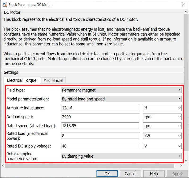
We have considered 'Permanent Magnet' field type and the model parameterization based on 'Rated Load and Speed'.
No-load speed is set to 2400 RPM whereas Rated speed is set to 1818.95 RPM.
Rated load(Mechanical Power) is set to 8 kW and the motor is energized by a 48 V DC power supply.
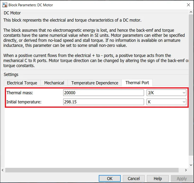
Since we have enabled the thermal port, it is necessary to determine the thermal mass and the initial temperature of the DC motor.The thermal mass is set to 20000 J/K from the default value of 100 J/K, whereas the initial temperature is kept default at 298.15 K or 25 C.
Thermal mass represents the energy required to raise the temperature of the thermal port by one degree.Hence by increasing the thermal mass to a value of 20000 J/K, 20000 Joules heat has to be absorbed by the DC motor for its temperature to rise by 1 K.
The reason for increasing the thermal mass to a very high value of 20000 J/K is to improve the performance of the DC motor.
The increase in motor temperature results in the increase in the winding resistance and decrease in the magnetic flux.The increase in winding resistance results in the increase in no-load speed beyond safe limits and also due to the decrease in magnetic flux the torque output reduces drastically.This ultimately causes the efficiency of the motor to degrade.
Upto to a certain temperature limit, the permanent magnets are subject to partial demagnetization, which on cooling can be reversed.But beyond critical limits, the magnets may loose their magnetization permanently.
Hence by increasing the thermal mass to a very high value, we can reduce the rate of rise in temperature of the DC motor.
Thus by constraining the DC motor to operate within the safe temperature limits we can prevent the degradation in the performance and efficiency of the DC motor.
Current Sensor : The Current Sensor block represents an ideal current sensor, that is, a device that converts current measured in any electrical branch into a physical signal proportional to the current.Connections + and – are electrical conserving ports through which the sensor is inserted into the circuit. Connection I is a physical signal port that outputs the measurement result.
With reference to this model :
The + and - terminals of the block are connected with the + and - terminals of the DC motor.This block helps us in determining the current drawn by the DC motor.The physical signal generated by this block is connected to the 'Battery Module' sub-system which in turn helps us in determing the State of Charge of the battery.
Temperature Sensor : The Temperature Sensor block represents an ideal temperature sensor, that is, a device that determines the temperature differential measured between two points without drawing any heat.Connections A and B are thermal conserving ports that connect to the two points where temperature is being monitored. Port T is a physical signal port that outputs the temperature differential value.The block positive direction is from port A to port B. The measured temperature is determined as -
T = TA – TB.
With reference to this model : There are two temperature sensors used in the model and they are connected as follows -
- The A port is connected to the thermal port of the H-bridge, whereas the B port is connected to a thermal reference. The physical signal (T port) generated is used to determine the temperature of the motor controller(H-bridge).
- The A port is connected to the thermal port of the DC motor, whereas the B port is connected to a thermal reference. The physical signal (T port) generated is used to determine the temperature of the DC motor.
Mechanical Rotational Reference : This block represents a reference point, or frame, for all mechanical rotational ports. All rotational ports that are rigidly clamped to the frame (ground) must be connected to a Mechanical Rotational Reference block.
With reference to this model :
The Casing (C port) of the DC motor is connected to this block.
Electrical Reference : This block represents an electrical ground. Electrical conserving ports of all the blocks that are directly connected to ground must be connected to an Electrical Reference block. A model with electrical elements must contain at least one Electrical Reference block.
With reference to this model :
All the negative terminals of the electrical blocks used in the sub-system are connected to the Electrical Reference.Also the Reference ports of the Controlled Voltage Source and H-Bridge blocks are connected to this block.Since we have not considered using the DC motor for reverse motion of the electric car, we have connected the REV port of the H-bridge to the Electrical Reference.
Thermal Reference : This block represents a thermal reference point, that is, a point with an absolute zero temperature, with respect to which all the temperatures in the system are determined.
Solver Configuration : Each physical network represented by a connected Simscape block diagram requires solver settings information for simulation.This specifies the solver parameters that our model needs before we can begin simulation.Each topologically distinct Simscape block diagram requires exactly one Solver Configuration block to be connected to it.
Battery Module
Battery : This block implements a generic dynamic model that represents most popular types of rechargeable batteries.
The block provides predetermined charge behavior for four battery types. For the lithium-ion battery, the block provides models for simulating temperature and aging effects.
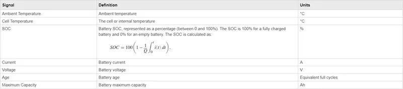
Output vector of signals for the battery temperature, state-of-charge, current, voltage, age, maximum capacity, and the ambient temperature is determined by the block.
There are a few assumptions with respect to this mode and they are as follows :
-
The internal resistance is assumed to be constant during the charge and discharge cycles and does not vary with the amplitude of the current.
-
The parameters of the model are derived from the discharge characteristics. The discharging and charging characteristics are assumed to be the same.
-
The capacity of the battery does not change with the amplitude of the current (there is no Peukert effect).
-
The self-discharge of the battery is not represented. It can be represented by adding a large resistance in parallel with the battery terminals.
-
The battery has no memory effect.
With reference to this model :
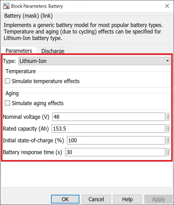
We have opted for a lithium-ion battery.The temperature and aging effects of the batttery have not been considered.
The nominal voltage is considered to be 48 V and the rated capacity to be 153.5 Ah.The initial state of charge is considered to be 100 % and the battery response time to be 30 seconds.
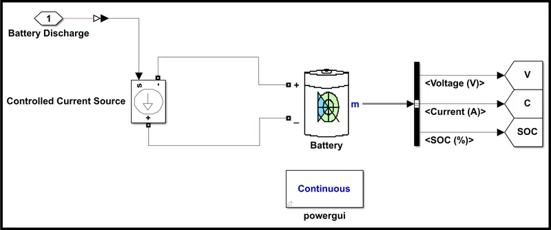
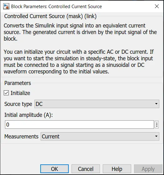
Controlled Current Source (SIMULINK) : Converts the Simulink input signal into an equivalent current source. The generated current is driven by the input signal of the block.You can initialize your circuit with a specific AC or DC current. If you want to start the simulation in steady-state, the block input must be connected to a signal starting as a sinusoidal or DC waveform corresponding to the initial values.
With reference to this model : The source type is set to DC and the initial amplitude is kept default at 0 A.The measurements dropdown is set to currents.A multimeter block can be placed in the model to display the selected measurements during the simulation.
The current signal from the DC motor is connected to the physical signal port of this block.The positive and negative terminals of this block are connected to the reverse polarities of the battery.
Powergui : The powergui block allows us to choose one of these methods to solve your circuit:
-
Continuous, which uses a variable-step solver from Simulink®
-
Discretization of the electrical system for a solution at fixed time steps
-
Continuous or discrete phasor solution
The powergui block also opens tools for steady-state and simulation results analysis and for advanced parameter design.
We need the powergui block to simulate any Simulink model containing Simscape™ Electrical™ Specialized Power Systems blocks. It stores the equivalent Simulink circuit that represents the state-space equations of the model.
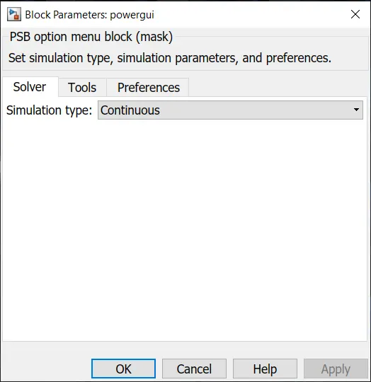
With reference to this system : The simulation type of the block is set to continuous.
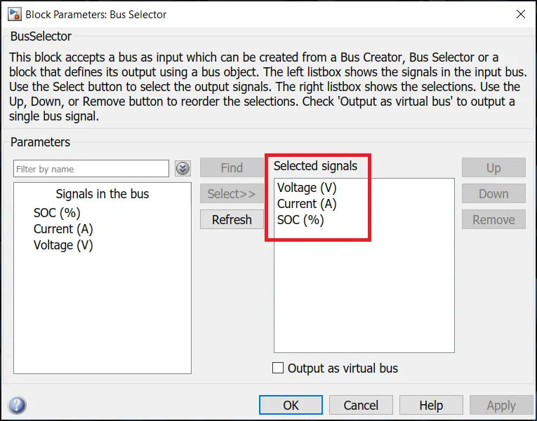
Bus Selector : This block accepts a bus as input which can be created from a Bus Creator, Bus Selector or a block that defines its output using a bus object. The left listbox shows the signals in the input bus. The Select button is used to select the output signals. The right listbox shows the selections. Use the Up, Down, or Remove button to reorder the selections. Check 'Output as virtual bus' to output a single bus signal.
With reference to this model : The Voltage, Current and SOC vector signals from the battery have been selected in the Bus Selector to be represented as output.
Vehicle Body
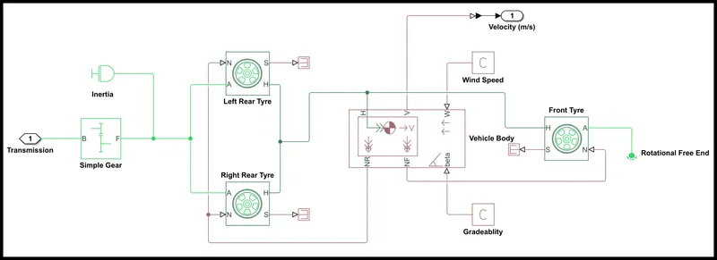
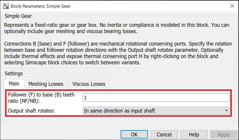
Simple Gear : This block represents a gearbox that constrains the connected driveline axes of the base gear, B, and the follower gear, F, to co-rotate with a fixed ratio that we specify. We have an option to choose whether the follower axis rotates in the same or opposite direction as the base axis. If they rotate in the same direction, the angular velocity of the follower, ωF, and the angular velocity of the base, ωB, have the same sign. If they rotate in opposite directions, ωF and ωB have opposite signs.
With reference to this model :
We have set the Gear Ratio to 1 and ensured that the ouput shaft rotates in the same direction as the input shaft.
The meshing and viscous losses have been set to be default.
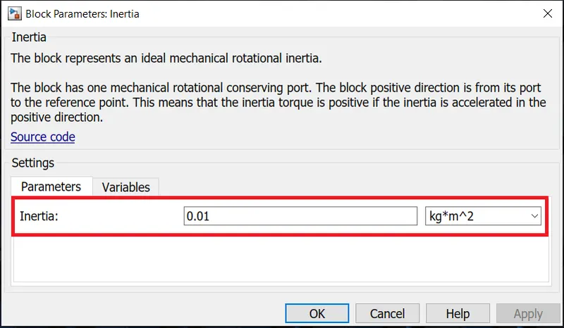
Inertia : This block represents an ideal mechanical rotational inertia, described with the following equation:
`T = J*(domega)/dt`
where T = Inertia Torque
J = Inertia
`omega` = Angular Velocity
t = Time
The block has one mechanical rotational conserving port. The block positive direction is from its port to the reference point. This means that the inertia torque is positive if inertia is accelerated in positive direction.
With reference to this model :
This block is connected to the Follower (F) output of the Simple Gear block.
We have set the inertia value to 0.01 kg`m^2`.
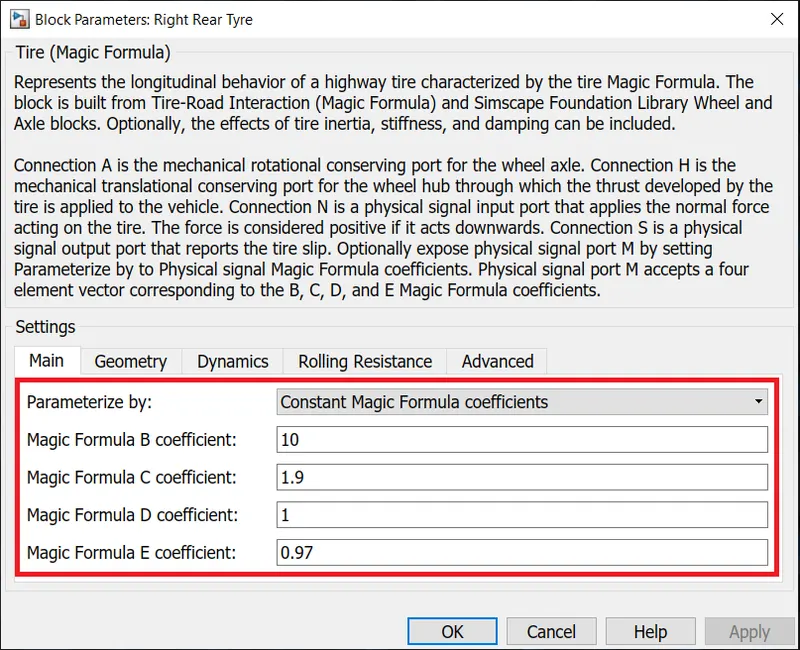
Tire (Magic Formula) : The Tire (Magic Formula) block models a tire with longitudinal behavior given by the Magic Formula, an empirical equation based on four fitting coefficients. The block can model tire dynamics under constant or variable pavement conditions.The longitudinal direction of the tire is the same as its direction of motion as it rolls on pavement.
To increase the fidelity of the tire model, we can specify properties such as tire compliance, inertia, and rolling resistance. However, these properties increase the complexity of the tire model and can slow down simulation. Hence we consider ignoring tire compliance and inertia while simulating the model in real time or while preparing the model for hardware-in-the-loop (HIL) simulation.
Connection A is the mechanical rotational conserving port for the wheel axle. Connection H is the mechanical translational conserving port for the wheel hub through which the thrust developed by the tire is applied to the vehicle. Connection N is a physical signal input port that applies the normal force acting on the tire. The force is considered positive if it acts downwards. Connection S is a physical signal output port that reports the tire slip.
With reference to this model :
We have set the parameterization type to 'Constant Magic Formula Coefficients'.
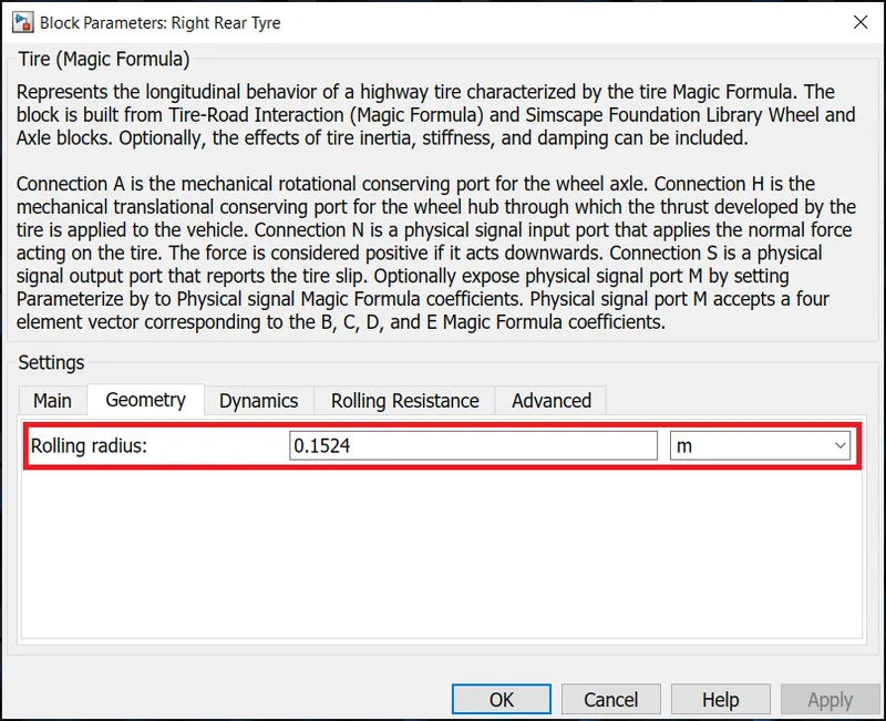
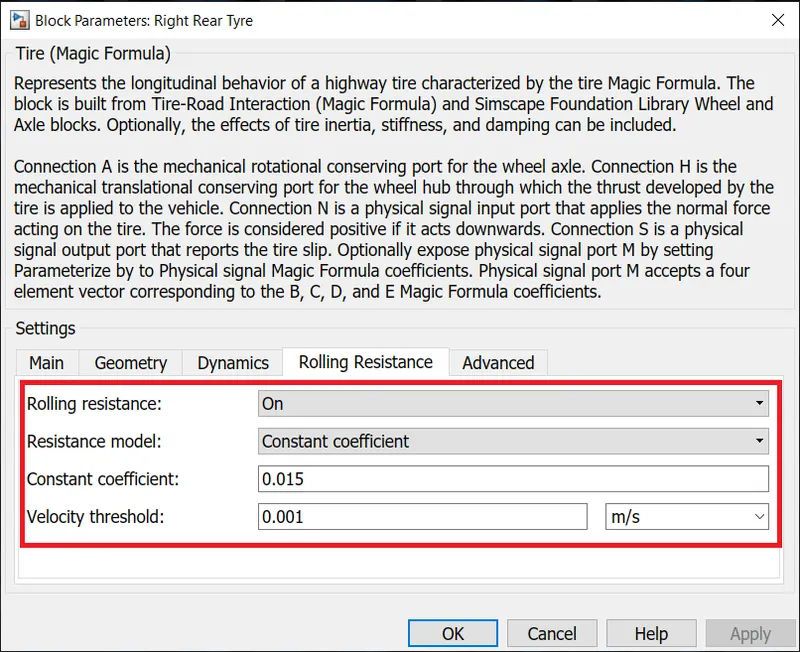
We have set the Rolling Radius to be 0.1524 m and turned on Rolling Resistance option with default settings.
Vehicle Body : The Vehicle Body block represents a two-axle vehicle body in longitudinal motion. The vehicle can have the same or a different number of wheels on each axle. For example, two wheels on the front axle and one wheel on the rear axle. The vehicle wheels are assumed identical in size. The vehicle can also have a center of gravity (CG) that is at or below the plane of travel.The block accounts for body mass, aerodynamic drag, road incline, and weight distribution between axles due to acceleration and road profile. Optionally include pitch and suspension dynamics. The vehicle does not move vertically relative to the ground.The block has an option to include an externally-defined mass and an externally-defined inertia. The mass, inertia, and center of gravity of the vehicle body can vary over the course of simulation in response to system changes.
Connection H is the mechanical translational conserving port associated with the horizontal motion of the vehicle body. The resulting traction motion developed by tires should be connected to this port. Connections V, NF, and NR are physical signal output ports for vehicle velocity and front and rear normal wheel forces, respectively. Wheel forces are considered positive if acting downwards. Connections W and beta are physical signal input ports corresponding to headwind speed and road inclination angle, respectively.
With reference to this model :
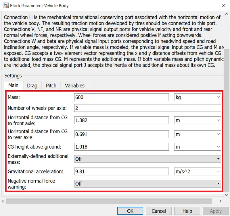
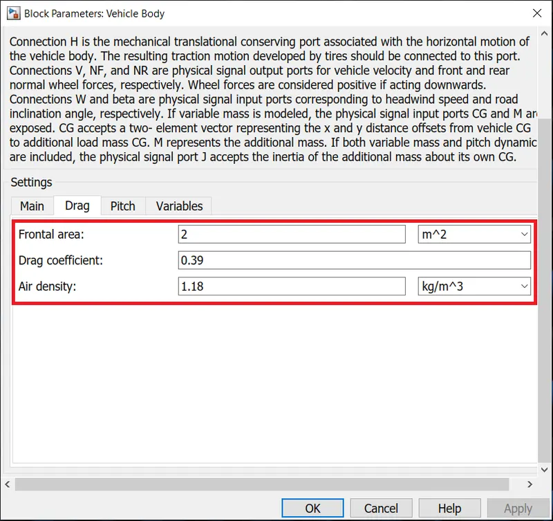
We have considered the Head Wind Speed to be 1.67 m/s and the Road Inclination to be 0 radians.
The rest of the parameters are provided with values as shown in the images below.
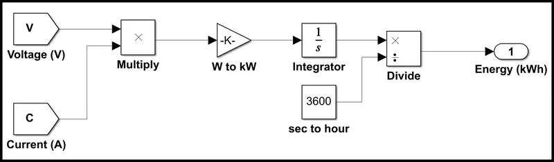
Energy Calculation Sub-system
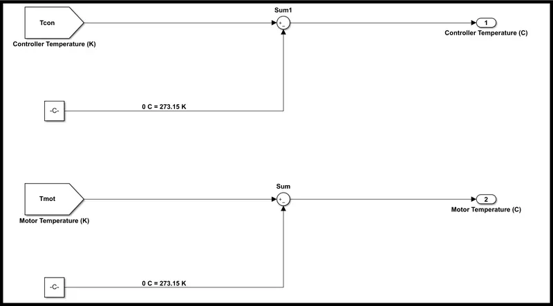
Temperature Unit Conversion (K to C) Sub-system
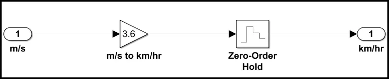
Vehicle Velocity Conversion (m/s to km/hr) Sub-system
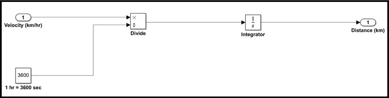
Distance (km) Calculation Sub-system
RESULTS
Case 1 : The drive cycle used for the simulation is FTP-75.
Drive-Cycle Speed v/s Vehicle Speed in m/s
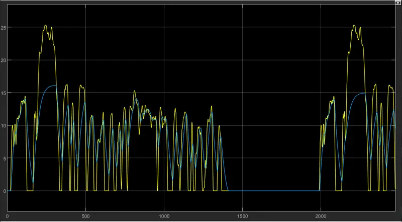
Yellow Line : Drive Cycle Speed (m/s)
Blue Line : Actual Vehicle Speed (m/s)
From the above graph it is evident that the vehicle falls behind the drive cycle.Since the design parameters of the DC motor used in the vehicle is very much constrained to that of an ideal electric rickshaw, the vehicle is not able to achieve the steep acceleration and deceleration as depicted in the FTP-75 drive cycle.The vehicle can attain speeds only upto 16 m/s or 57.6 km/hr.
Energy Consumption in kWh
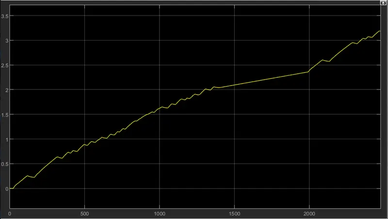
The energy consumption at the end of the drive cycle is 3.20 kWh, almost half of the total battery capacity.Such high consumption of energy is due to the fact that there are frequent instances of acceleration and deceleration in the FTP-75 drive cycle.
Motor Controller Temperature v/s Motor Temperature in K
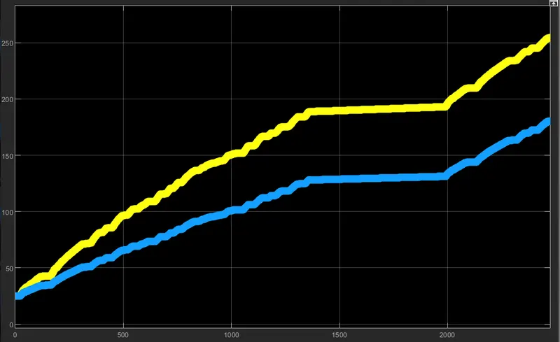
Yellow Line : Motor Controller Temperature (C) = 250 C
Blue Line : DC Motor Temperature (C) = 180 C
Battery State Of Charge (SOC) in %
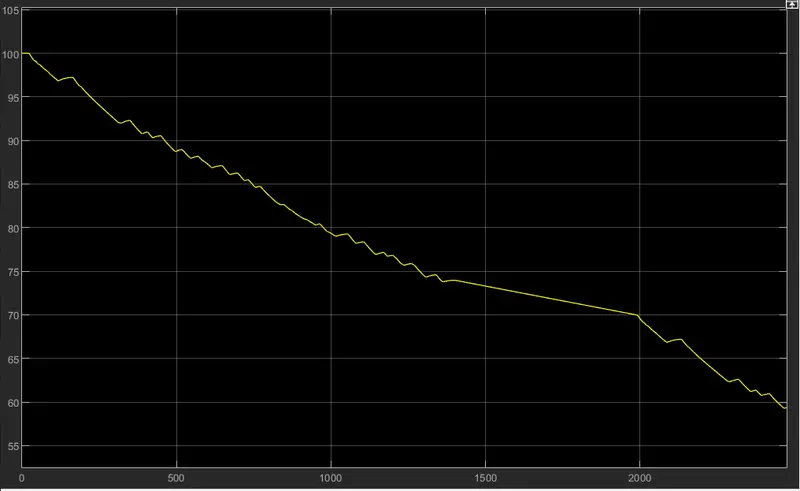
At the end of the drive cycle the battery SOC has dropped to 59.5 %.It can be observed from the graph that there are numerous instances where the battery has recharged, which is due to regenerative braking.
Case 2 : The drive cycle used for the simulation is EUDC.
Drive-Cycle Speed v/s Vehicle Speed in m/s
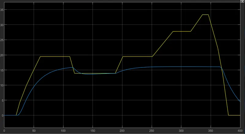
Yellow Line : Drive Cycle Speed (m/s)
Blue Line : Actual Vehicle Speed (m/s)
From the above graph it is evident that the vehicle falls behind the drive cycle.Since the design parameters of the DC motor used in the vehicle is very much constrained to that of an ideal electric rickshaw, the vehicle is not able to achieve the steep acceleration and deceleration as depicted in the EUDC drive cycle.The vehicle can attain speeds only upto 16 m/s or 57.6 km/hr.
Energy Consumption in kWh
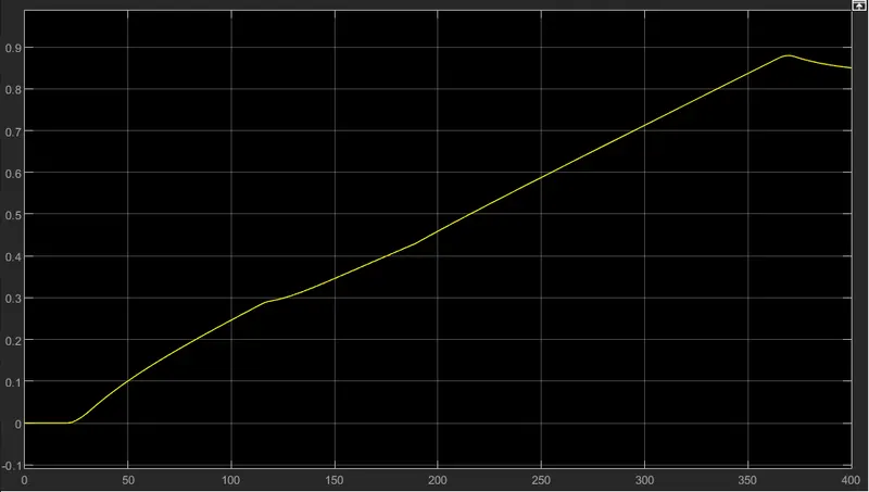
The energy consumption at the end of the drive cycle is 0.85 kWh.Compared to the previous drive cycle the energy consumption in EUDC drive cycle is very less, since the duration of the drive cycle is very less compared to the previous one and also due to the fact that this drive cycle is not subjected to frequent acceleration and decelration.
Motor Controller Temperature v/s Motor Temperature in K
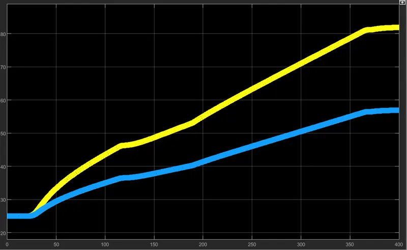
Yellow Line : Motor Controller Temperature (C) = 82 C
Blue Line : DC Motor Temperature (C) = 57 C
Battery State Of Charge (SOC) in %
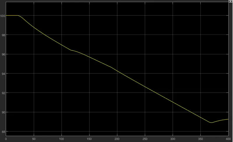
At the end of the drive cycle the battery SOC has dropped to 89.25 %.The SOC in this cycle is comparitively greater than the previous one, since this drive cycle is of short duration and is not subject to frequent change in speeds.
Case 3 : The drive cycle used for the simulation is UDDS.
Drive-Cycle Speed v/s Vehicle Speed in m/s
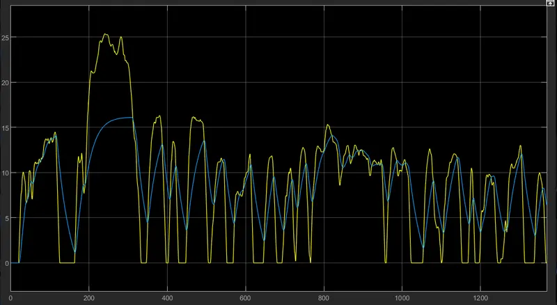
Yellow Line : Drive Cycle Speed (m/s)
Blue Line : Actual Vehicle Speed (m/s)
From the above graph it is evident that the vehicle falls behind the drive cycle.Since the design parameters of the DC motor used in the vehicle is very much constrained to that of an ideal electric rickshaw, the vehicle is not able to achieve the steep acceleration and deceleration as depicted in the UDDS drive cycle.The vehicle can attain speeds only upto 16 m/s or 57.6 km/hr.
Energy Consumption in kWh
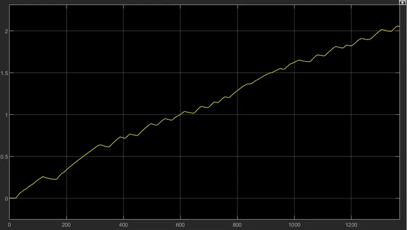
The energy consumption at the end of the drive cycle is 2.05 kWh.
Motor Controller Temperature v/s Motor Temperature in K
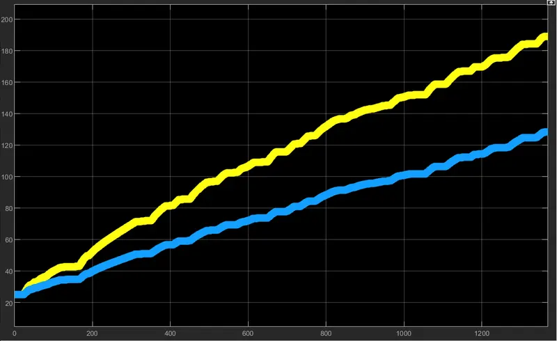
Yellow Line : Motor Controller Temperature (C) = 189 C
Blue Line : DC Motor Temperature (C) = 128 C
Battery State Of Charge (SOC) in %
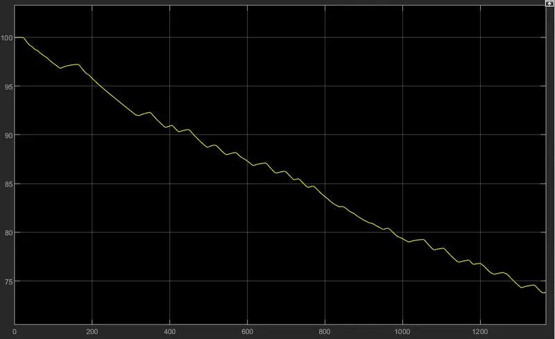
At the end of the drive cycle the battery SOC has dropped to 73.75 %.It can be observed from the graph that there are numerous instances where the battery has recharged, which is due to regenerative braking.