Week 4 - Genetic Algorithm
AIM : To optimise stalagmite function and to find the global maxima of the function.
THEORY :
Optimisation : It is a decision making process where the best results are obtained from a set of input values under prioritised constraints.The set of all possible solutions or values which the inputs can take make up the search space. In this search space, lies a point or a set of points which gives the optimal solution. The aim of optimization is to find that point or set of points in the search space.
There are two methods under optimisation
- Deterministic Approach : In this model all the parameter values and initial conditions are available to determine output with certainity.
- Stochastic Approach : This model possess some inherent randomness.It is a probabilistic method.This means that the same set of parameter values and initial conditions will lead to an ensemble of different outputs.
Genetic Algorithm : Genetic Algorithms (GAs) are search based algorithms based on the concepts of natural selection and genetics. GAs are a subset of a much larger branch of computation known as Evolutionary Computation.
In GAs, we have a pool or a population of possible solutions to the given problem. These solutions then undergo crossover and mutation , producing new solutions, and the process is repeated over various iterations. Each solution is assigned a fitness value and the fitter solutions are given a higher chance to mate and yield more optimised solutions.This process continues till the stopping criteron is reached.This is in line with the Darwinian Theory of Survival of the Fittest.
Advantages
- Useful when the search space is very large and there are a large number of parameters involved.
- Does not require any derivative information.
- It is faster and more efficient as compared to the traditional methods.
Disadvantages
- GAs are not suited for problems where derivative information is available.
- Being stochastic, there are no guarantees on the optimality or the quality of the solution.
- Since fitness value is calculated repeatedly it might be computationally expensive for some problems.
Applications
- Neural Networks
- Image Processing
- Machine Learning
- Robot Trajectory Generation
- Economics
Basic terminologies invloved
- Population : It is a subset of all the possible solutions to the given problem.
- Chromosomes : It is is one such solution to the given problem.
- Gene : It is one element position of a chromosome.
- Allele : It is the value a gene takes for a particular chromosome.
- Genotype : It is the population in the computation space.
- Phenotype : It is the population in the actual real world solution space.
- Encoding : It is the process of transforming a solution from phenotype to genotype space.
- Decoding : It is the process of transforming a solution from genotype to phenotype space.
GOVERNING EQUATIONS :
The stalagmite function is defined by a parameter :
f(x,y) = `f1,x*f1,y*f2,x*f2,y`
where
f1,x = `[sin(5.1*pi*x + 0.5)]^6`
f1,y = `[sin(5.1*pi*y + 0.5)]^6`
f2,x = `exp[ (-4*ln(2)) * (x - 0.0667)^2 /0.64 ]`
f2,y = `exp[ (-4*ln(2)) * (y - 0.0667)^2 /0.64 ]`
PROGRAM : The code is written using MATLAB.
Main Program :
% Genetic Algorithm Code

clear all
close all
clc

% Defining our search space
x = linspace(0,0.6,150) ;
y = linspace(0,0.6,150) ;
num_cases = 50 ;

% Creating a 2 Dimensional Mesh
[xx yy] = meshgrid(x,y) ;

% Evaluating the stalagmite function
for i = 1:length(xx)
    for j = 1:length(yy)
        input_vector(1) = xx(i,j) ;
        input_vector(2) = yy(i,j) ;
        f(i,j) = stalagmite_func(input_vector) ;
    end
end

tic
% Study 1 : Statistical behaviour with unbounded inputs
for i = 1:num_cases
    [inputs fopt(i)] = ga(@stalagmite_func,2) ;
    xopt(i) = inputs(1) ;
    yopt(i) = inputs(2) ;
end
Study1_time = toc

% Plotting Study 1
figure(1)
subplot(2,1,1)
surfc(x,y,f)
shading interp
hold on
plot3(xopt,yopt,fopt,'marker','o','markersize',5,'markerfacecolor','r')
title('Ubounded Inputs')
xlabel('X-Axis')
ylabel('Y-Axis')
subplot(2,1,2)
plot(fopt)
xlabel('Iterations')
ylabel('Function Maximum')

tic
% Study 2 : Statistical behaviour with upper and lower bounded inputs
for i = 1:num_cases
    [inputs fopt(i)] = ga(@stalagmite_func,2,[],[],[],[],[0;0],[0.6;0.6]) ;

    xopt(i) = inputs(1) ;
    yopt(i) = inputs(2) ;
end
Study2_time = toc

% Plotting Study 2
figure(2)
subplot(2,1,1)
surfc(x,y,f)
shading interp
hold on
plot3(xopt,yopt,fopt,'marker','o','markersize',5,'markerfacecolor','r')
title('Bounded Inputs')
xlabel('X-Axis')
ylabel('Y-Axis')
subplot(2,1,2)
plot(fopt)
xlabel('Iterations')
ylabel('Function Maximum')

tic
% Study 3 : Statistical behaviour with increased GA iterations
options = optimoptions('ga') ;
options = optimoptions(options,'PopulationSize',200) ;

for i = 1:num_cases
    [inputs fopt(i)] = ga(@stalagmite_func,2,[],[],[],[],[0;0],[0.6;0.6],[],[],options) ;
    xopt = inputs(1) ;
    yopt = inputs(2) ;
end
Study3_time = toc

% Plotting Study 3
figure(3)
subplot(2,1,1)
surfc(x,y,f)
shading interp
hold on
plot3(xopt,yopt,fopt,'marker','o','markersize',5,'markerfacecolor','r')
title('Bounded Inputs with Increased Population Size ')
xlabel('X-Axis')
ylabel('Y-Axis')
subplot(2,1,2)
plot(fopt)
xlabel('Iterations')
ylabel('Function Maximum')
Stalagmite Program :
% Stalagmite Function

function Maxima = stalagmite_func(input_vector)
x = input_vector(1) ;
y = input_vector(2) ;
f1x = (sin((5.1*pi*x) + 0.5))^6 ;
f1y = (sin((5.1*pi*y) + 0.5))^6 ;
f2x = exp((-4*log(2))*(((x - 0.0667)^2)/(0.64))) ;
f2y = exp((-4*log(2))*(((y - 0.0667)^2)/(0.64))) ;
Maxima = -(f1x*f1y*f2x*f2y) ;
end
OUTPUT :
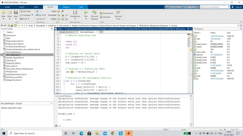
PLOTS :
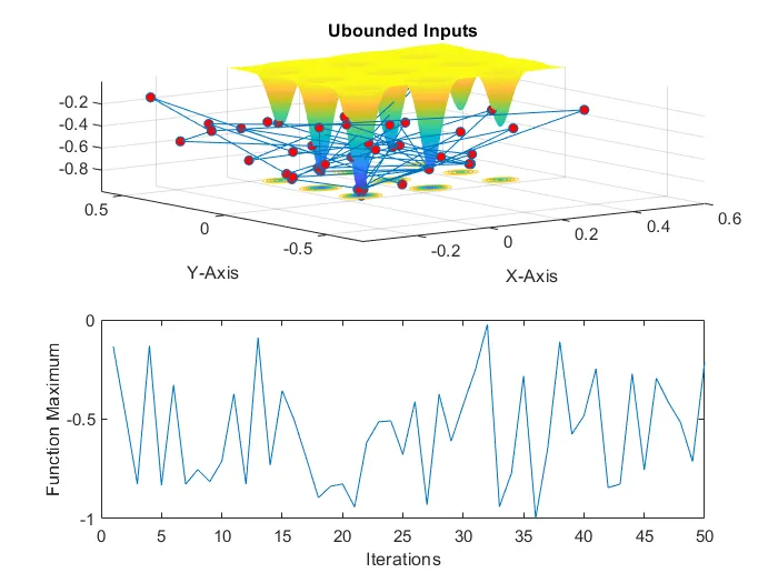
STUDY 1 : Statistical behaviour with unbounded inputs.
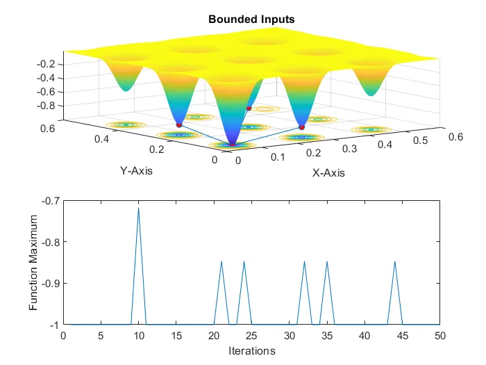
STUDY 2 : Statistical behaviour with lower and upper bounds.
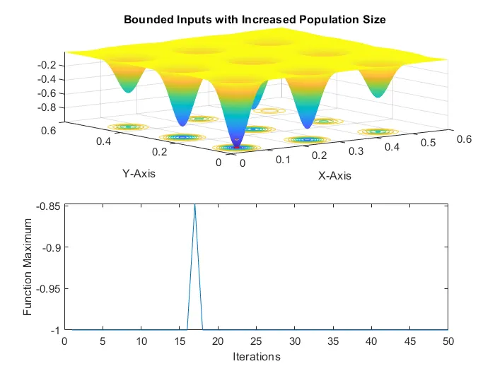
STUDY 3 : Statistical behaviour with bounded inputs using increased GA iterations.
EXPLANATION :
- We begin our program by defining the search space and also by assigning the number of cases for the loop to be run through.
- Further we create a 2 dimensional array using 'meshgrid' command.
- Now using the 'for loop' we determine the number loops the 'input_vector' has to be run through.The output 'f(i,j)' is determined using a stalagmite function.
- The stalagmite_func is written on the basis of parameters mentioned under 'GOVERNING EQUATIONS'.
- Under 'Study 1' we create another 'for loop' to obtain the optimal solutions using genetic algorithm.This loop is run for a fixed number of cases.
- Now the statistical behaviour is studied by plotting the above formulated output.We begin by assigning the figure number.Now 'subplot' command is used to create numerous plots under the same figure.Moving on we use 'surfc(x,y,z)' command to create a surface.'Shading interp' command is used so that the grid lines are not displayed on the surface generated.
- Carrying on we use the 'plot3' to create a 3D plot.The input values and the optimal solution are plotted as markers.
- Now under another subplot the optimal solution as a function of number of iterations is plotted for easy analyzation of the optimal values varying at each iteration.
- Similarly the above procedure is followed for 'Study 2' and 'Study 3' and the results are generated by only tweaking the syntax for genetic algorithm (ga) in the program code.
GENETIC ALGORITHM SYNTAX :
X = GA(PROBLEM) finds the minimum for PROBLEM. PROBLEM is a structure that has the following fields:
X = GA(FITNESSFCN,NVARS,Aineq,bineq,Aeq,beq,lb,ub,NONLCON,INTCON,options)
FITNESSFCN: <Fitness function>
NVARS: <Number of design variables>
Aineq: <A matrix for inequality constraints>
bineq: <b vector for inequality constraints>
Aeq: <Aeq matrix for equality constraints>
beq: <beq vector for equality constraints>
lb: <Lower bound on X>
ub: <Upper bound on X>
NONLCON: <Nonlinear constraint function>
INTCON: <Index vector for integer variables>
options: <Options created with optimoptions('ga',...)>
rngstate: <State of the random number generator>
[X,FVAL] = GA(FITNESSFCN, ...) returns FVAL, the value of the fitness
function FITNESSFCN at the solution X.
REFERENCES :