Rayleigh Taylor Instability Challenge
What are some practical CFD models that have been based on the mathematical analysis of Rayleigh Taylor waves? In your own words, explain how these mathematical models have been adapted for CFD calculations
The Rayleigh Taylor Instability arises when a high density fluid is placed over a low density fluid in a gravity field. When the density interface is disturbed, the hydrostatic pressure is generated, so the heavier fluid moves downwards and mixes with the lighter one, with the amplitude of pertubation initially growing exponentially but after some time saturates and forms a characteistic mushroom shape. When a heavier fluid is displaced downward with an equal volume of lighter fluid is displaced upwards, it results in decrease of potential energy than its initial state.
Practical CFD models that have been based on mathematical analysis of Rayleigh Taylor waves are:
1. Ritchmeyer Meshkov Instability:-The Richtmyer–Meshkov instability (RMI) occurs when two fluids of different density are impulsively accelerated. Normally this is by the passage of a shock wave. The development of the instability begins with small amplitude perturbations which initially grow linearly with time. This is followed by a nonlinear regime with bubbles appearing in the case of a light fluid penetrating a heavy fluid, and with spikes appearing in the case of a heavy fluid penetrating a light fluid. A chaotic regime eventually is reached and the two fluids mix. This instability can be considered the impulsive-acceleration limit of the Rayleigh Taylor instability.
Following the deposition of vorticity at the contact surface, the resultant flow is an example of a time dependent decaying inhomogenous mixing layer. The impinging shock wave imparts a velocity impulse and deposits vorticity at the interface. Following the linear phase the single mode instability develops into mushroom shaped ring vortices in three dimensions or vortex pairs in two dimensions. Flow field evolves as a decaying turbulent mixing layer.
Due to time consuming nature of fully 3D simulation, it is desirable to run 2D simulation where possible. The governing equations involve solving two dimensional Euler equations where both speceis are assumed to be in pressure and velocity equilibrium and viscosity is assumed to be negligible. Shock waves and material interfaces must be resolves hence a very high order finite volume method is employed
2.Kelvin Helmholtz instability is a hydrodynamic instability in which immiscible, incompressible, and inviscid fluids are in relative and irrotational motion. In KHI, the velocity and density profiles are uniform in each fluid layer, but they are discontinuous at the (plane) interface between the two fluids. This discontinuity in the (tangential) velocity, i.e., the shear flow, induces vorticity at the interface; as a result, the interface becomes an unstable vortex sheet that rolls up into a spiral
2. Perform the Rayleigh Taylor instability simulation for 2 different mesh sizes with the base mesh being 0.5 mm. Compare the results by showing the animations( Attach them from your google drive). Observe the differences in the animation and explain the effect of mesh size on simulation. Also, explain why a steady-state approach might not be suitable for these types of simulation.[ Choose Air and Water for this simulation]
Setting up of Geometry
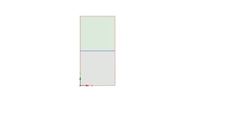
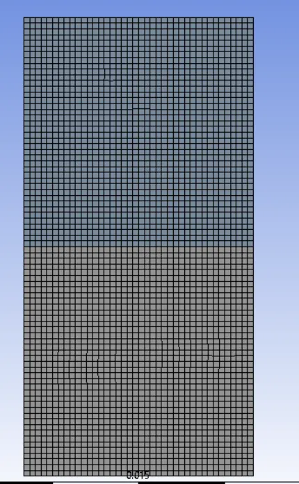
Two square surfaces of side 20 mm representing air and water were created. Denser element water represents the upper surface while the rarer surface water represents the lower surface. Topology was set to share.
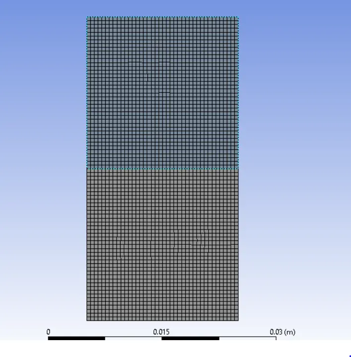
A mesh with elemet size of 0.5mm was generated. The number of nodes were 3321 and element 3200

Setup
1) General-1) Pressure Based Solver
2) Transient Time step
3) Gravity enabled- value set to -9.81m/s^2
2) Physics- 1) Laminar model has been used
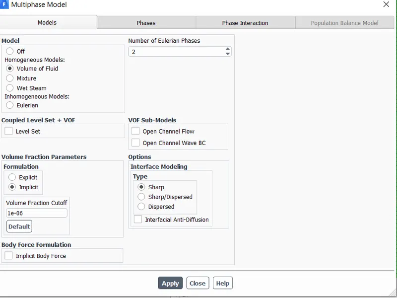
2) Multiphase- Volume of Fluid used with no of eulerian phases set to 2
3) air set as the primary phase, water set as the secondary phase
3) Solution Methods
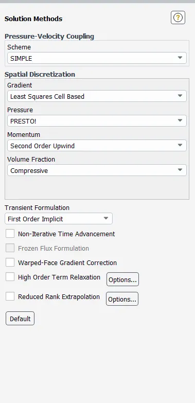
5) Solution is then initialized
6) After initializiation domain is Patched. Volume fraction of water is set to 1 in Water and 0 in air surface
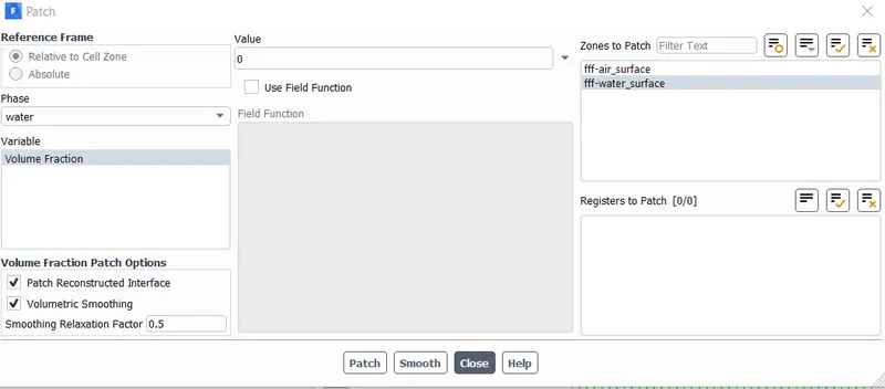
7) Using a time step of 0.005 solution is run for 1500 iterations.
Results
i) Case 1- Base Mesh 0.5mm
a) Mesh: No of Nodes- 3321
No of Elements-3200
ii) Evolution of instability with time steps
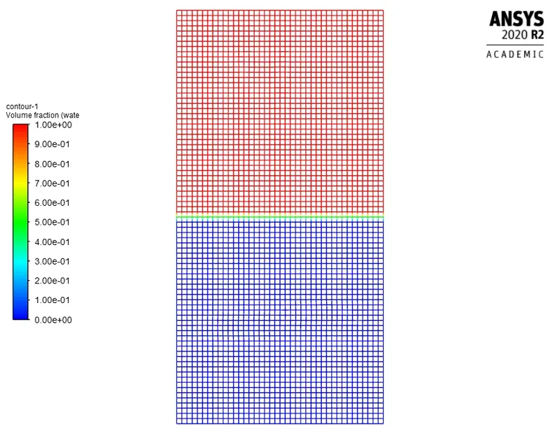
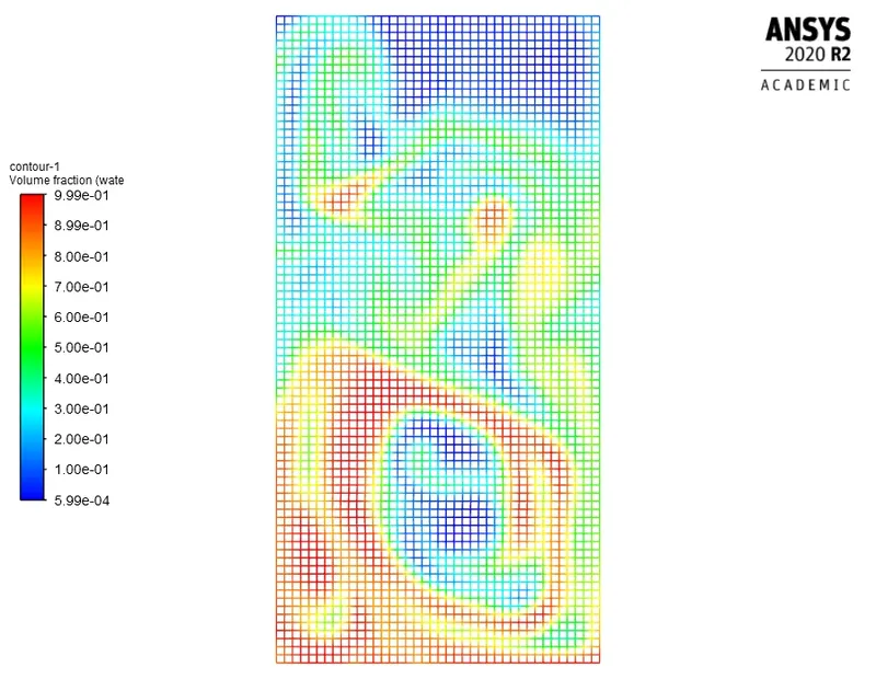
t=0 t=100
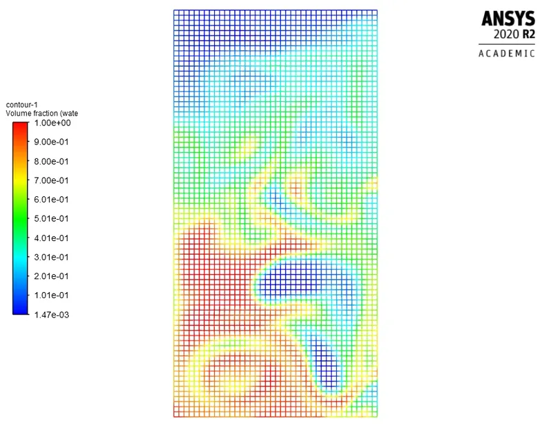
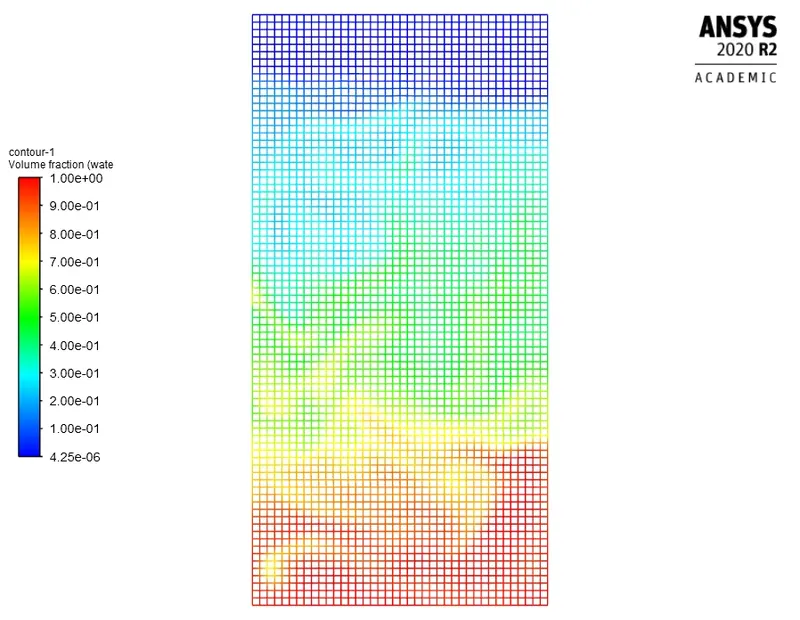
t=120 t=300
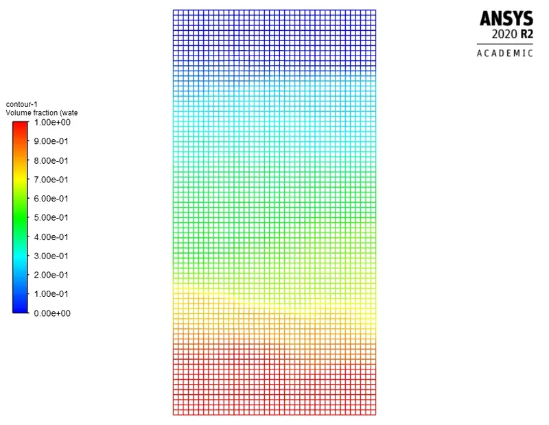
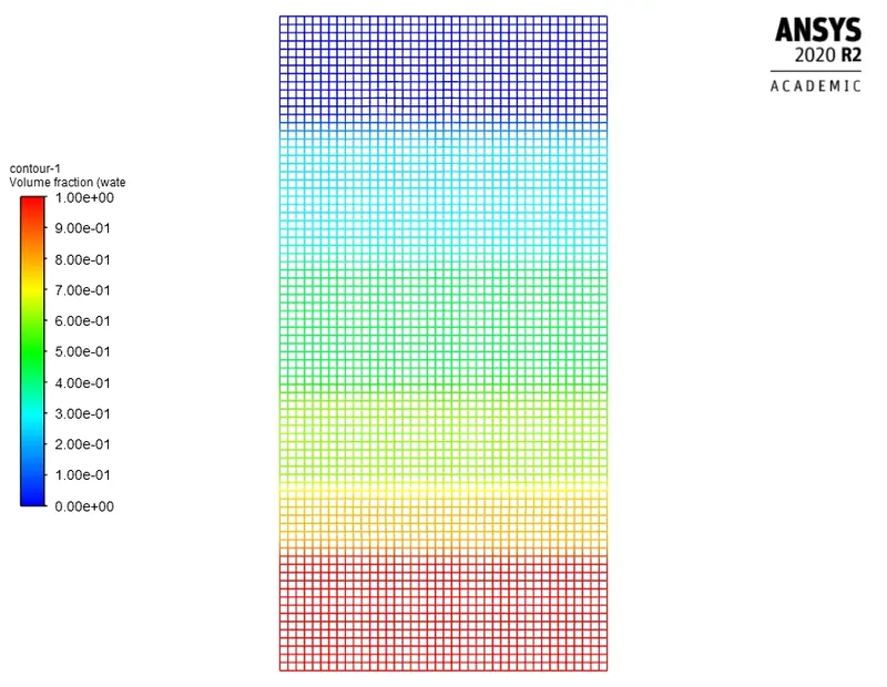
t=500 t=1000
iii) Animation
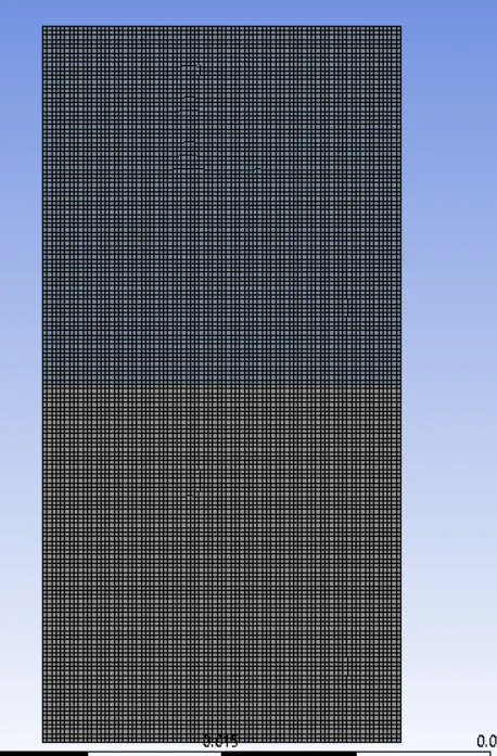
b) Case 2-Refined Mesh 0.25mm
i) Mesh:- Nodes- 13041
Elements- 12800
ii) Evolution of Instability over time step
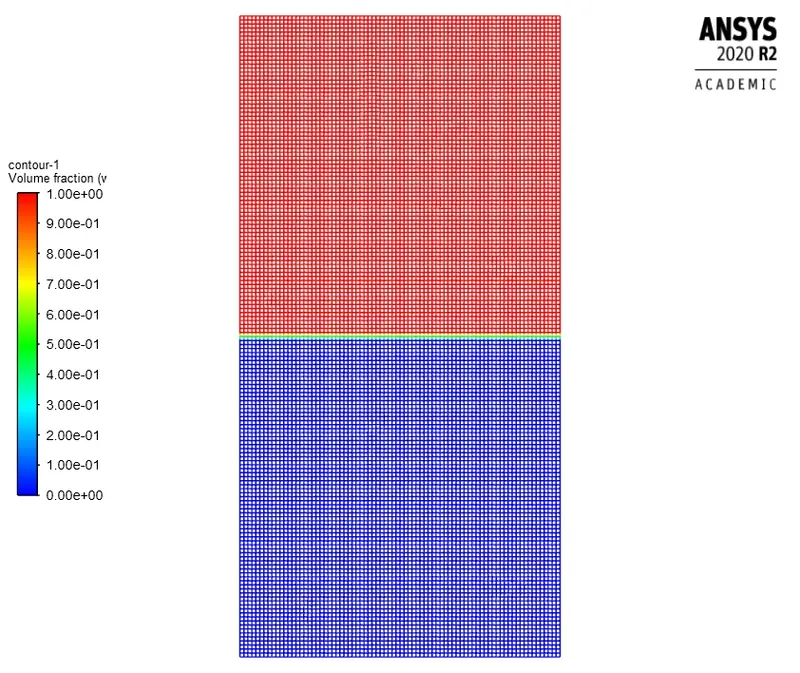
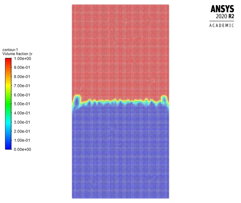
t=0 t=8
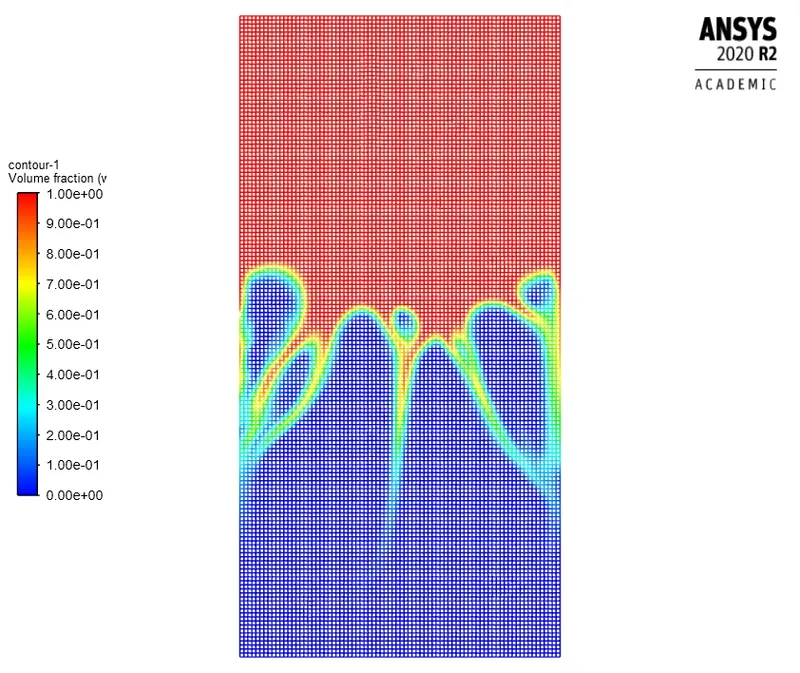
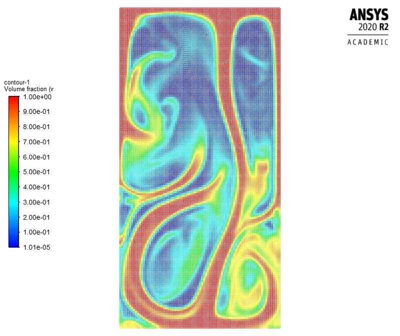
t=50 t=122
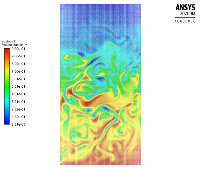
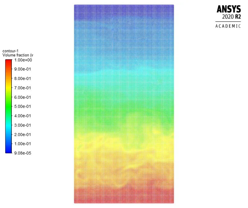
t=350 t=400
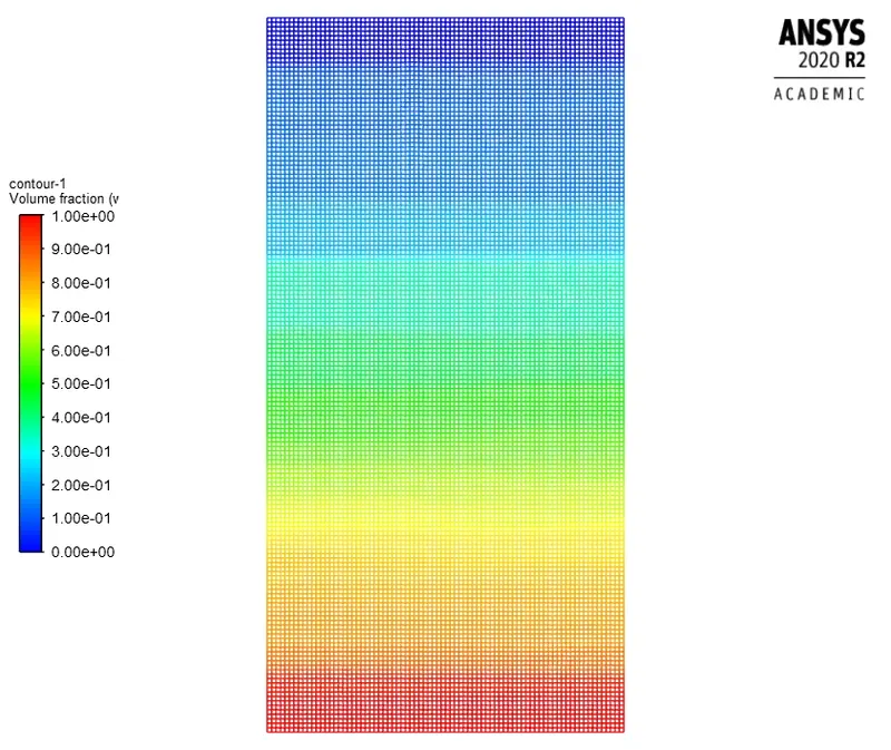
t=1000
iii) Animations
Observation:- We note that the simulation starts with a state of hydr0static equilibrium. As the mesh is refined we are able to observe the development of deformation more clearly. In the end of the simulation the two phases get separated from each other with some diffusivity in the middle regions.
Whether Steady state apporoach would be suitable
Since the instabilities evolve over time a steady state simulation would not give a correct representation. Steady state would be more suitable if we are concerned about equilibrium state.
3. Simulation using User defined mesh
i) Mesh Nodes- 13041
Elements- 12800
ii) Evolution of instability with time
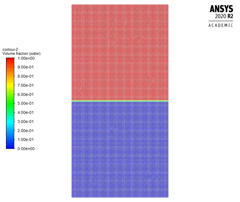
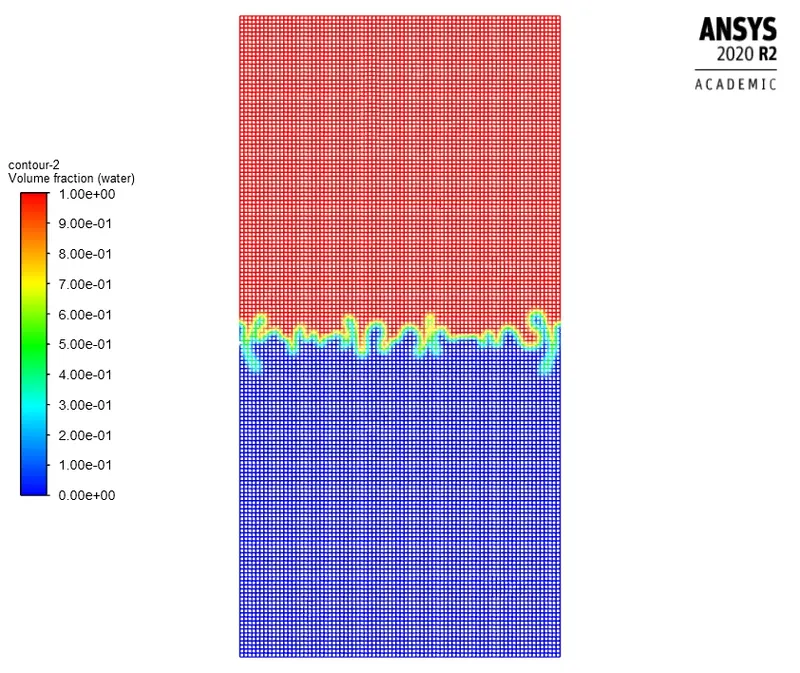
t=0 t=40
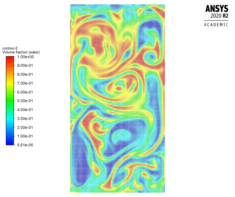
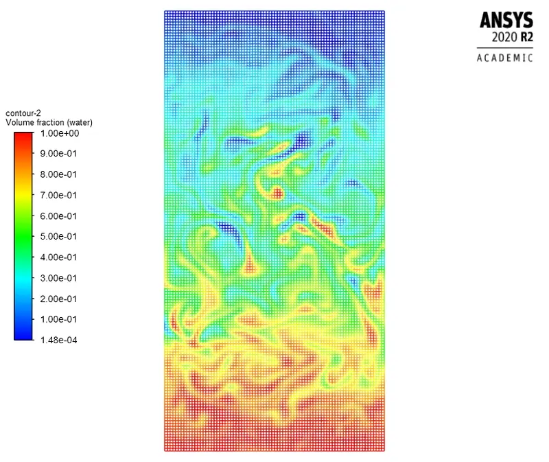
t=150 t=200
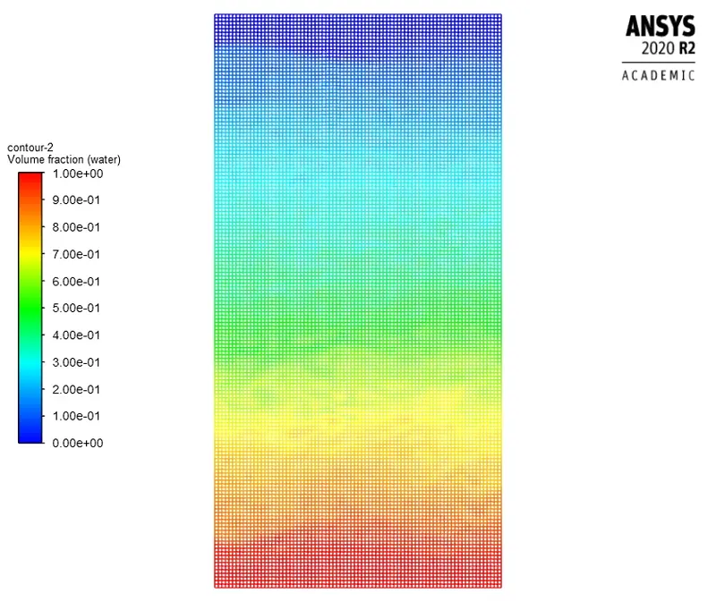
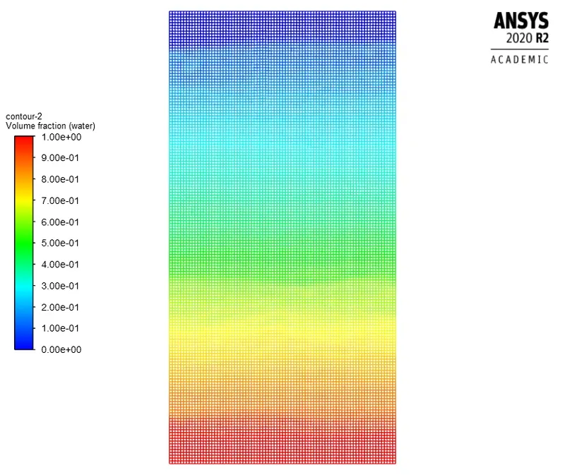
t=400 t=1000
iii) Animations
Simulation-User defined material
4) Define the Atwood Number. Find out the Atwood number for both the cases and explain how the variation in Atwood number in the above two cases affects the behavior of the instability.
The Atwood number (A) is a dimensionless number in fluid dynamics used in the study of hydrodynamic instabilities in density stratified flows. It is a dimensionless density ratio defined as

where
 = density of heavier fluid
 = density of lighter fluid
Atwood number for air-water case
A= (998.2-1.225)/(998.2+1.225)=0.9975
Atwood number for water-user defined case
A= (998.2-400)/(998.2+400)=0.427
It is seen that with larger Atwood number larger amplitude of peturbations are observed. Due to the large density ratio, stronger is the force to develop the interface instability.
For the case of small Atwood number, the density difference between the two sides of the interface is small, and the density distribution of the upper and lower layers is nearly symmetrical. The initial density stratification plays a dominant role, and the expansion-compression effect has little influence. With the increase in the Atwood number, the stabilization effect of initial density stratification decreases, and the instability caused by the expansion-compression effect becomes more significant